
Split Ring Resonator
Abstract
The advent of metamaterials has represented a paradigm shift in how engineers design new electromagnetic devices and even media with unusual properties. One canonical example of a metamaterial is the split ring resonator, the first to experimentally verify the possibility of a negative refractive index. This example shows how to simulate a split ring resonator using metamaterials with a negative refractive index near 11 GHz using Ansys HFSS.
The retrieved material parameters are extracted from the first design as datasets and then used in two other designs to create equivalent and simpler models. In addition to the vacuum region, the simplified design contains only a monolithic cube of equivalent material, with the detailed geometry (substrate and conductors) of the split ring resonator excluded.
This example model document is available from the HFSS online help and from the PDF included with the example model in the software installation (accessible from the Project Manager when this example project is open).
Simulation Time / RAM: (meshing, adaptive solution, and frequency sweep in 2025 R1, 6 cores with 64 GB RAM)
- 1_Original: 5 minutes: 20 seconds with 2.76 GB max. memory used per process
- 2_Complex_Equiv_Matl: 42 seconds with 206 MB max. memory used per process
- 3_Equiv_Matl_Using_Loss_Tangent: 40 seconds with 206 MB max. memory used per process
The equivalent material approach is much faster and, if used with a more complex design, the benefit in RAM and solution time will be even greater.
Introduction
The split ring resonator is the classic example of a metamaterial that can achieve negative refractive index. First verified experimentally in 2001 [1], much of the motivation for development of such materials can be attributed to the prospect of a “perfect lens” [2]. However, many other interesting applications have been identified in the last decade.
Since metamaterials are usually complex composite structures, analytical solutions to their scattering properties quickly become unfeasible. Therefore, numerical simulation is a crucial step in the design process. In this example, we show how to model and analyze a split ring resonator [3] in Ansys HFSS. The example shows some of the most important points of metamaterial simulation and characterization, including the boundary and port definitions, solution setup, and even effective parameter retrieval.
Model Construction and Setup Details
Design 1_Original:
Only the first design (1_Original) contains the split ring resonator substrate and conductor geometry. For the two subsequent designs, a simple cube of equivalent material, with parameters extracted from the first design, is substituted for the split ring resonator assembly.
Using the geometric parameters in Ref. [3], the geometry of the split ring resonator was modeled in HFSS. Given the relative simplicity of the structure, there are several valid ways to draw it. In this case, we first started with a box to represent the FR4 substrate. Next, polylines were drawn to trace out the metallic pieces on both sides of the substrate, which were then thickened to the desired conductor dimensions by setting the Cross Section to “Rectangle” and specifying the desired variables for the width and height of the traces.
After drawing the substrate, resonator, and wire structures, a region was added to define the boundaries of the computational domain. This region is important so that the correct unit cell size along x and y is defined, and so that the ports can be placed sufficiently away from the near-fields induced on the structure. This region size ensures that the scattering parameters are calculated properly. The resulting geometry is shown below:
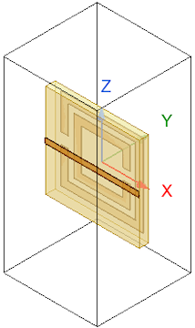
Figure 1: Design 1_Original Geometry
Coupled Lattice Pair Boundaries and Floquet Port Excitations
After drawing the geometry and defining the materials, the next step was to assign boundaries and excitations. Since we modeled a single unit cell, which is to be situated in a periodic lattice, coupled Lattice Pairs are the correct choice for the boundaries on the ±x and ±y faces of the model domain:
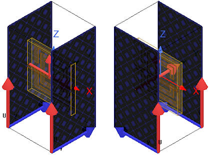
Figure 2: Coupled Lattice Pair Boundaries
Floquet ports were then added as excitations to the ±z faces of the model domain:
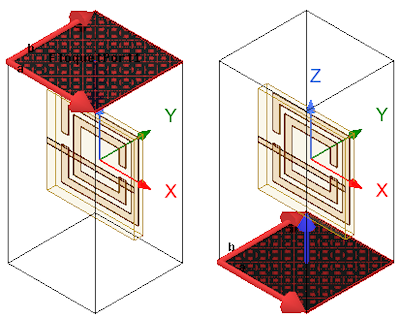
Figure 3: Floquet Port Excitations
A crucial setting worth noting for the Floquet ports in this case is the de-embedding. Since accurate calculation of the S-parameter phase is important for effective parameter retrieval, the ports must be de-embedded to the surface of the unit cell, as indicated by the blue arrows in the above figures.
Mesh Settings and Operations:
To ensure higher quality elements, the Mesh Method has been set to TAU for all three designs. Additionally, because the thin solid conductors in the first design (1_Original) are more problematic than the simple box features of the other two designs, the following mesh operations were defined for the first design only. These operations provide the desired element sizes and help to ensure the success of the TAU mesh:
- Length-Based, On Selection: 0.1 mm Maximum Length
- Surface Representation Priority for TAU: High (assigned to all conductors)
Setup:
All three designs have a single adaptive solution frequency of 11 GHz specified and an interpolated frequency sweep from 1–20 GHz in 0.05 GHz steps. Only the convection criteria differ. Design 1_Original allows more adaptive passes (20 maximum versus 15 for the other two) and a relaxed Delta S value (0.02 versus 0.01 for the other two). The differing convergence criteria ensure successful solving of the more complex geometry of the first design. For all three solutions, two consecutive converged steps must be achieved.
Effective Material Parameter Retrieval in HFSS
Perhaps the most important and difficult step in metamaterial analysis is retrieval of the effective material parameters from the frequency-dependent S-parameters obtained by the simulation or scattering experiment. Thanks to the Output Variables functionality, it is possible to perform this step in HFSS without having to export any data to an external script, though one may do so if desired.
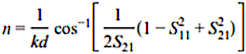
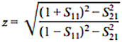
Ref. [3] gives the relevant equations needed for performing the effective parameter retrieval, specifically Equations 9 and 10:
In the Output Variables window for this example project (HFSS > Results > Output Variables), you will find the equations for the effective parameters used in HFSS. They are also shown below:
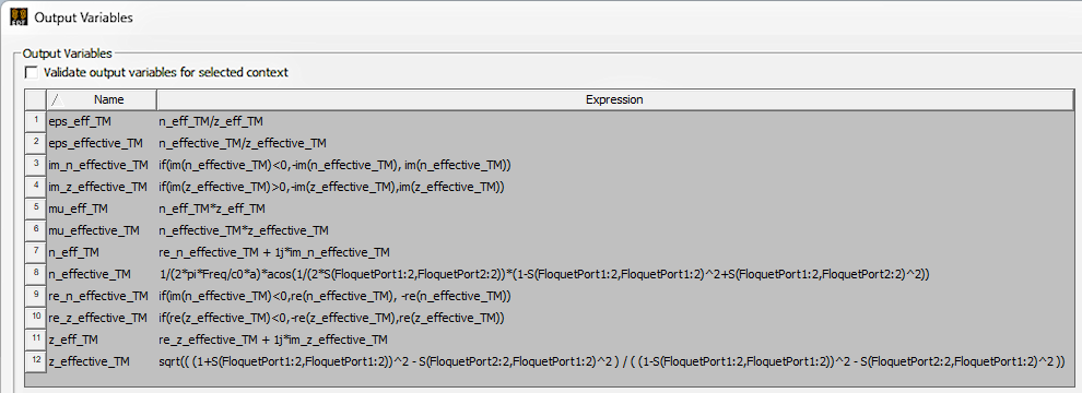
Figure 4: List of Defined Output Variables (All Designs)
Parameter retrieval is a complicated process, and some care must be taken when defining these equations for your projects. There are some conditional statements that are required to avoid discontinuities and to make the resulting effective parameters physically meaningful and passive. As an example, view the results below (Figures 5–8) for the retrieved parameters that were calculated before applying the required conditions, that is, naively applying Equations 9 and 10 from Reference [3].
Retrieved Material Parameters (before Applying Necessary Conditions):
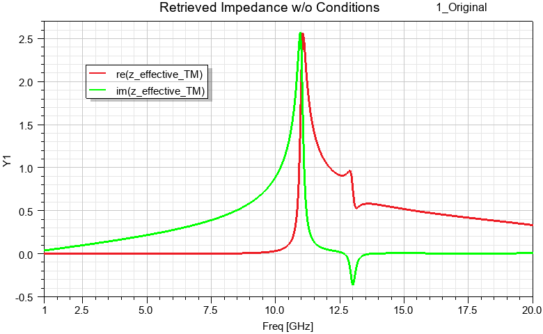
Figure 5: Retrieved Impedance Plot without Required Conditional Statements
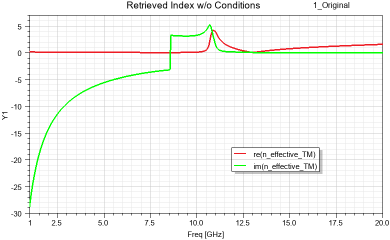
Figure 6: Retrieved Index Plot without Required Conditional Statements
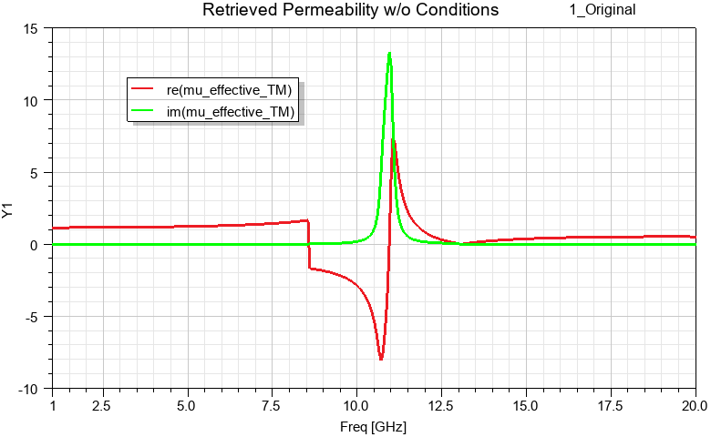
Figure 7: Retrieved Permeability Plot without Required Conditional Statements
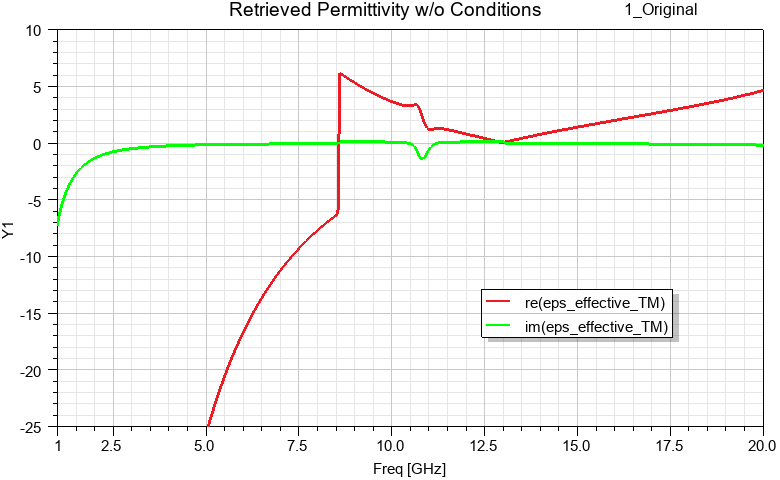
Figure 8: Retrieved Permittivity Plot without Required Conditional Statements
Note the unphysical discontinuities in the preceding retrieved index, permeability, and permittivity plots. Additionally, there is clearly an issue with the signs of the retrieved index and impedance. These clues indicate that we have not calculated physical and passive material parameters.
Next, variables with the conditional statements required to correct the retrieved parameters were used as the basis of a second set of plots. The final results showing the correct retrieved parameters follow (Figures 9–12).
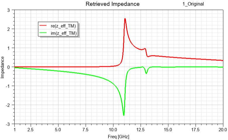
Figure 9: Retrieved Impedance Plot after Applying Conditional Statements
The following figure confirms the negative sign of the real part of the refractive index (red trace) near resonance:
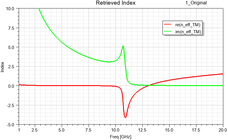
Figure 10: Retrieved Index Plot after Applying Conditional Statements
Also, the magnetic resonance of the structure is clearly visible from the following retrieved permeability figure:
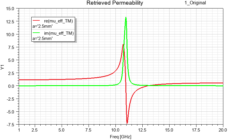
Figure 11: Retrieved Permeability Plot after Applying Conditional Statements
It may appear strange that there is an antiresonance in the negative, imaginary part of the retrieved permittivity (the green trace in the following figure). However this can be attributed to the fact that the homogenization limit has not quite been reached. More details are given in the text of Reference [3]:
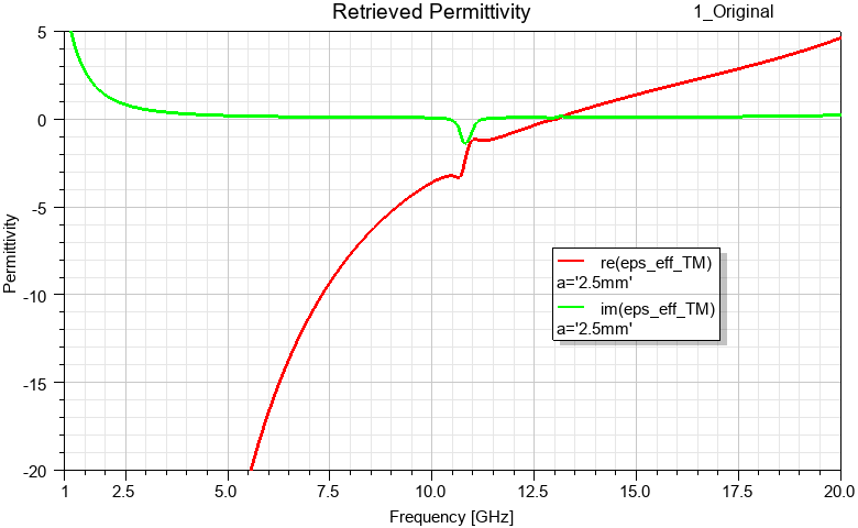
Figure 12: Retrieved Permittivity Plot after Applying Conditional Statements
Constructing an Equivalent Material from the Retrieved Properties:
- Right-click inside one of the retrieved parameter plot windows and choose Export from the shortcut menu. Use the default CSV format.
- Import the CSV as a project dataset so that it is available to all designs in the project:
- From the menu bar, click Project > Datasets.
- In the Datasets dialog box that appears, click Import.
- Browse to and select the exported CSV file and click Open.
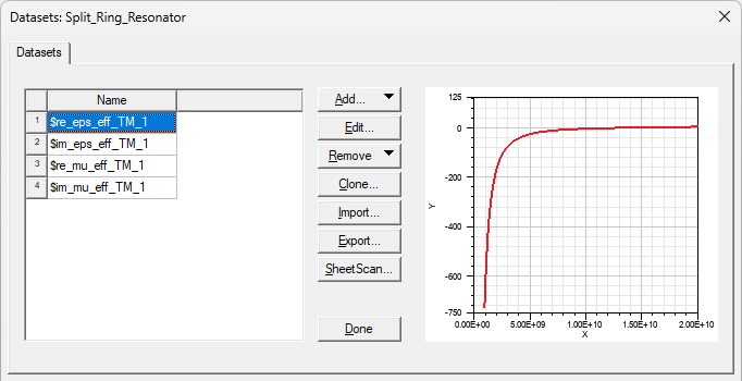
Figure 13: Datasets Dialog Box
As an illustration of the two different ways to define equivalent material properties, two equivalent designs have been built:
- Design 2_Complex_Equiv_Matl uses a complex equivalent material based on a complex definition for permittivity and permeability.
- Design 3_Equiv_Matl_Using_Loss_Tan uses a material based on real values for permittivity and permeability but with the dielectric and magnetic loss tangents defined.
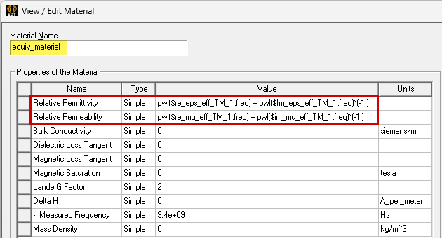
Figure 14: Complex Equivalent Material Properties – Used in Design 2
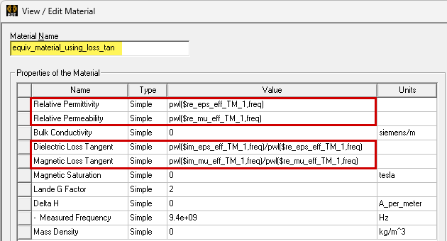
Figure 15: Equivalent Material with Loss Tangent Properties – Used in Design 3
Alternative Metamaterial Designs:
Now that we have the proper metamaterial properties, they can be used in designs 2_Complex_Equiv_Matl and 3_Equiv_Matl_Using_Loss_Tan. Both of these designs substitute a monolithic cube of metamaterial for the detailed geometry of the split ring resonator substrate and conductive traces.
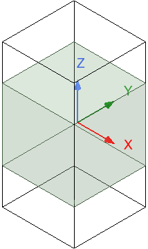
Figure 16: Metamaterials Model Geometry – Used in Designs 2 and 3
Post Processing
For each design, the Results branch of the Project Manager lists the available predefined plots. All three designs contain plots of the retrieved metamaterial properties—impedance, index, permeability, and permittivity. Additionally, each includes an S Parameters plot (S12). For this plot, trace data from the second and third designs has been copied to the first design's plot to directly compare S12 results between the original split ring resonator design and the equivalent metamaterial designs. After analyzing the setup, double-click any of these entries to display the associated plot. The retrieved material parameter plots have already been covered in the description of the retrieval process.
In this section we will look at a mesh overlay on the second design, to show the relative coarseness of the mesh that provides good, converged results when using simplified geometry and metamaterials:
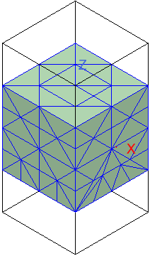
Figure 17: Equivalent Material's Mesh Overlay – Design 2
We will also look at comparative S Parameter results from all three designs to show how closely the metamaterials match the results of the original resonator geometry and conventional materials:
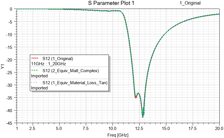
Figure 18: Comparison of S Parameter Results of all Three Designs
References:
[1] R. A. Shelby, D. R. Smith, S. Schultz, Science 292 (5514), 77-79 (2001).
[2] J. B. Pendry, Phys. Rev. Lett. 85, 3966-3969 (2000).
[3] D. R. Smith, D. C. Vier, Th. Koschny, C. M. Soukoulis, Phys. Rev. E 71, 036617 (2005).