
Potter Horn Antenna
Abstract
This example shows how to model a Potter Horn Antenna [1]. One design uses an FE-BI boundary, and another uses PML for its open region.
The horn is parametrized to facilitate the simulation of different geometry suited for various desired frequencies and gains. A frequency sweep from 28Ghz to 32Ghz is defined.
The model, Potter Horn Antenna.aedt, is available in the ...Examples/HFSS/Antennas folder under the Ansys Electronics Desktop software installation path. A PDF version of this topic is included with the project file in the same location.
Simulation Time: (meshing, adaptive solution, frequency sweep, and optimization in 2025 R1 using 6 cores and automatic HPC settings)
- Horn_Param_FEBI: 1 minute: 54 seconds, 791 MB max. memory per process
- Horn_Param_PML: 1 minute: 49 seconds, 1.67 GB max. memory per process
Model and Setup Details
The Potter Horn is a dual-mode feedhorn, which provides an excellent radiation pattern with suppressed sidelobes (at least 30 dB) and symmetrical beamwidths. The port at the small end of the model is excited at two modes, the fundamental TE11 mode and the TM11 second mode. The waves travel through a cylindrical guide (A in Figure 1) followed by taper (B). There is a step increase in diameter at the end of taper B. The two modes reach this step discontinuity with a relative amplitude and relative phase angle. The relative amplitudes of the two modes are controlled by the step, which converts a small percentage of the incident power from the TE11 mode to the TM11 mode, causing the E-Plane sidelobes to cancel. As the waves propagate through the phasing section (C), the relative phase angle is reduced prior to entering the flare (D). The length of section C is chosen so that the TE11 and TM11 modes are in phase when they reach the aperture.
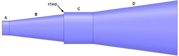
Figure 1: Potter Horn Diagram
The horn has w*λc wall thickness, and it is defined as aluminum. The port is internal to the solution region and is capped by a PEC object.
Details about the geometry and parameters can be seen in the History Tree and via HFSS > Design Properties (see Figure 2). This Potter Horn example has a very small flare angle (approximately 0.42°), as dictated by variables rC and rD:
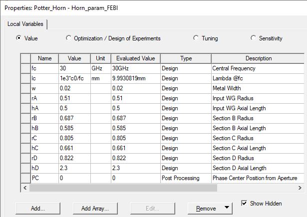
Figure 2: Horn Parameters
A Post Processing variable (PC) is defined to vary the position of the Far-field radiation coordinate system (Aperture_PC) along the z-axis for the phase center location calculation. The value of PC, the bottom variable in Figure 2, will change once the optimization analysis is complete.
This horn has been analyzed for the next Directivity values: 13, 15 and 20 dBi. These designs start with an input waveguide radius, rA=0.51λc and input Axial Length, hA=0.5λc. Starting with this dimension, an optimization within Ansys Optimization tools, quickly produces a design very close to the desired gain that radiates with low cross-polarization and very symmetrical radiation pattern. Table 1 shows Potter Horn Design Parameters (λc normalized):
| Gain (dBi) |
hD | rD | hC | rC | hB | rB | X-Pol Boresight (dB) |
10 dB Beamwidth (º) |
| 13.0 | 2.3 | 0.822 | 0.661 | 0.805 | 0.585 | 0.687 | -38 | 79.2 |
| 15.0 | 4.1 | 1.02 | 1.5 | 0.961 | 3.062 | 0.833 | -36 | 60.2 |
| 20.0 | 6.2 | 1.963 | 2.076 | 1.117 | 4.057 | 0.982 | -37.5 | 33.6 |
To set up any of these horns you only need to change the parameters described in Figure 2 and change the analysis setup to the desired frequency sweep range and increment.
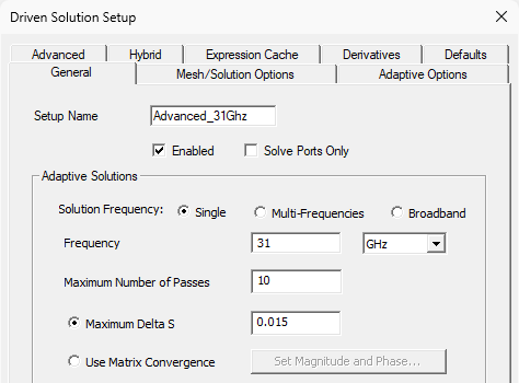
Figure 3 shows the analysis setup for the Potter Horn example (HFSS > Analysis Setup > Add Solution Setup > Auto). Figure 4 shows the frequency sweep setup (HFSS > Analysis Setup > Add Frequency Sweep). And Figure 5 shows the initial mesh settings that were specified (HFSS > Mesh > Initial Mesh Settings):
 |
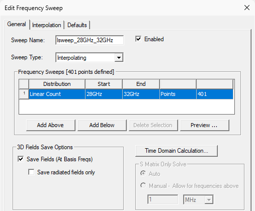 |
| Figure 3: Analysis Setup | Figure 4: Frequency Sweep Setup |
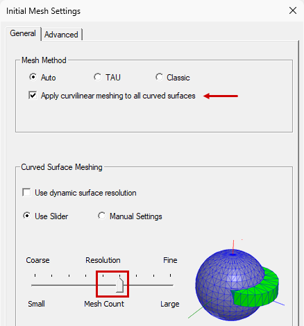
Figure 5: Initial Mesh Settings
Analysis Setup Notes:
- Either an FEBI- or PML-based absorbing boundary is a good choice for accurate directive antenna analysis.
- Advanced/Single-frequency adaptive solution is used here because the design is narrow band.
- In the Initial Mesh Settings: The Curvilinear option and finer than default curved surface meshing is used for increased accuracy for critical curved surfaces.
- Mesh seeding on the face of the absorbing boundary (to approximately λ/5) increases the accuracy of the far field pattern computation for a directive antenna. Only the face in the direction of the main beam is selected.
Both setups are automated. In the Modeler window, right-click and choose Create Open Region from the shortcut menu. Using PMLs is more efficient (faster) if multiple antennas or sources are present.
FEBI is mainly used when combined with hybrid boundaries (IE, PO, SBR+) to model electrically large environments, such as the antenna platform or radome.
The convergence criterion for delta S is 0.015. This value is a bit lower than the default of 0.02, since the return loss was expected to be very low (mainly below -30dB), and the additional accuracy has a negligeable effect on simulation time.
For highly complex geometry with many more curved faces (such as a non-simplified CAD model), curved surface meshing based on surface deviation can reduce the meshing complexity of non-critical and small sized curves.
When only interested in S parameters or analyzing a less directive antenna, this mesh refinement is not needed.
Postprocessing
After solving (Simulation > Analyze all), you can view different post-processing results. Look in the Project Manager under Results and double-click on the different predefined results (Figure 5):
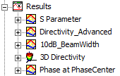
Figure 6: Post-Processing Results
In Appendix 1 you will find the FEBI version's predefined results obtained for a 13 dBi horn at 31 GHz (the adaptive solution frequency). S Parameters are plotted for the specified sweep frequency range of 28 to 32 GHz. Additionally, E-Field and 3D Directivity overlays are included. You can run the PML version and double-click the plots listed in the Project Manager for this version for comparison.
If you want to calculate the position of the phase center, please use the methodology defined in the Help Section: Determining Phase Center Using Optimetrics.
Once you simulate the horn alone you will be able to export it as a 3D Component (Draw > 3D Component Library > Create 3D Component) and simulate it as the feed of a reflector or quasi-optical system.
Appendix 1:
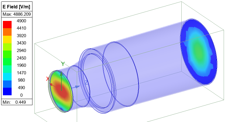
Figure 7: E-field @ Port 1 and Radiation Boundary (Aperture End) – FEBI Solution
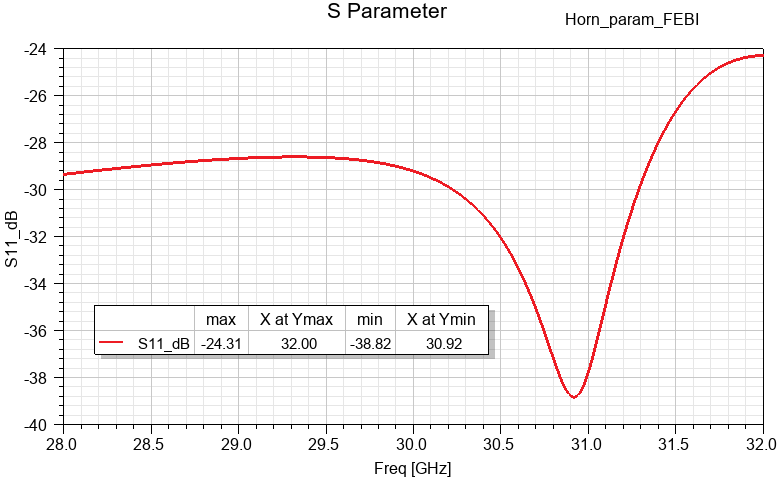
Figure 8: S Parameter vs. Frequency – FEBI Solution
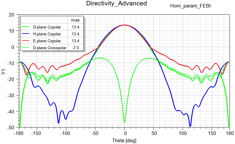
Figure 9: Directivity – FEBI Solution
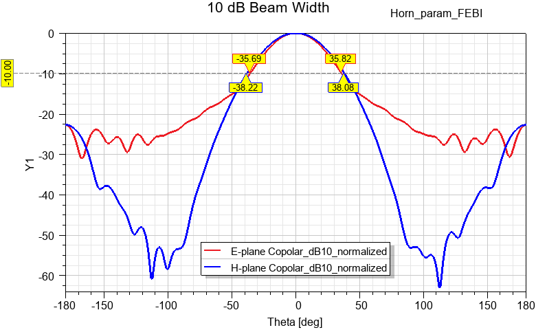
Figure 10: 10 dB Beam Width – FEBI Solution
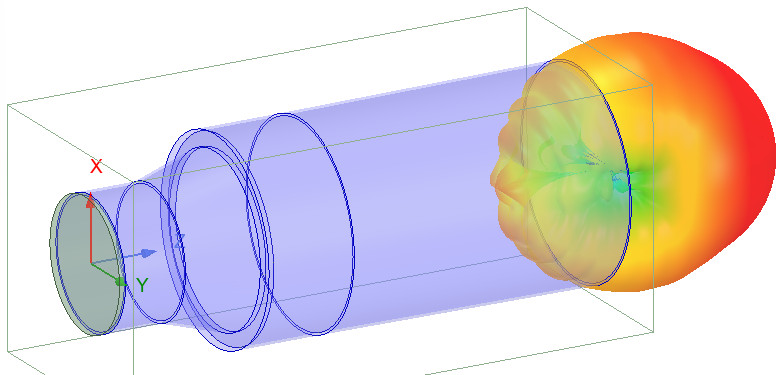
Figure 11: 3D Directivity Overlay – FEBI Solution
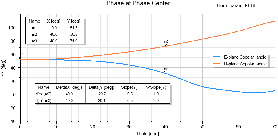
Figure 12: Phase at Phase Center – FEBI Solution
References:
[1] P. Potter, "A new horn antenna with suppressed sidelobes and equal beamwidths," Microwave Journal, pp. 71-78, June 1963.