Parabolic Dish with Horn

Abstract

A horn antenna with a parabolic dish for studying parametric placement of the horn along the dish's directional axis. This example also demonstrates usage of the mesh assembly option.

Solution Time: 14 cores in version 2025 R1 (meshing, adaptive solution, and parametric study)

System_IE: 40 minutes: 6 seconds, 4.31 GB max. memory per process
System_PO: 11 minutes: 50 seconds, 1.44 GB max. memory per process

Note:

Simulation time and memory will vary depending on your available resources. In most cases, HPC (parallel resources) can be leveraged to significantly reduce simulation time and the memory footprint required by each CPU.

Description:

This example shows an electrically large problem for the placement study of a horn antenna illuminating a dish when the antenna feed is moved along the X-axis. The horn and dish are defined as 3D Components to enable Mesh Assembly. Two projects are included for comparison, System_IE and System_PO, utilizing either an IE or PO region for the reflector. For such designs, meshing the horn and the dish separately makes the simulation faster since only the currents on the dish and on the radiation boundary of the horn need to be modeled. Meshing the volume of the region between the horn and the dish, to model coupling occurring due to the currents on the dish and the radiation volume bounding the horn, is not required. Additionally, with mesh assembly, you can reuse the meshes of the individual components for performing placement studies.

Simulation Summary:

For the best initial view of the model, choose the Trimetric view orientation rather than the default Isometric view. The curvature of the dish is more apparent from this viewpoint.

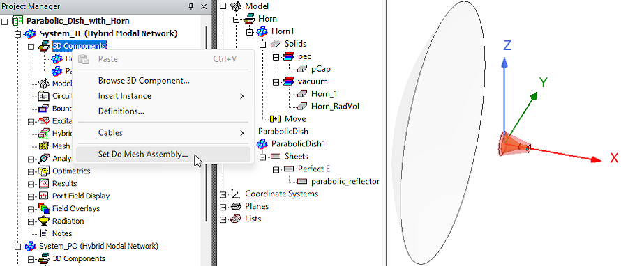
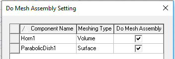
3D Components shortcut menu showing location of the Set Do Mesh Assembly option

The Parabolic Dish is 2 meters in diameter and is defined as a 3D Component with an IE or PO Hybrid Region assigned. The Horn is defined as a 3D Component with an FE-BI Region assigned. Both designs have the component option to Do Mesh Assembly enabled:

Do Mesh Assembly Setting dialog box

Solution Setup:

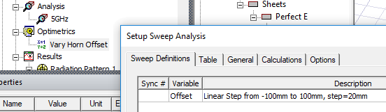
The adaptive solution frequency is 5 GHz. A design variable, Offset, is defined to vary the placement of the horn along the X axis for the Parametric Sweep setup ("Vary Horn Offset"):

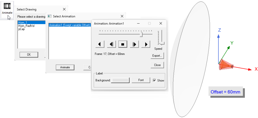
Sweep Definitions tab of the Setup Sweep Analysis dialog box, with settings for the Parametric solution.

Before solving a Parametric Sweep, you can use the Parametric Animation feature to see an animation of all the geometric variations that will be solved. Select the View tab of the Ribbon and click Animate. Then, in the Select Drawing dialog box, select Horn_1 and click OK. An animation is predefined with Offset defined as the swept variable. Click Animate to generate the frames and see the range of motion of the horn.

Accessing the Animation dialog box.

Solve both designs, one at a time, before proceeding to the postprocessing section. In the Project Manager, right-click on the design name and choose Analyze All from the shortcut menu to mesh the model, run the adaptive solution, the frequency sweep, and the parametric sweep.

Postprocessing

The example model includes two predefined plots and three field overlays per design, as listed below:

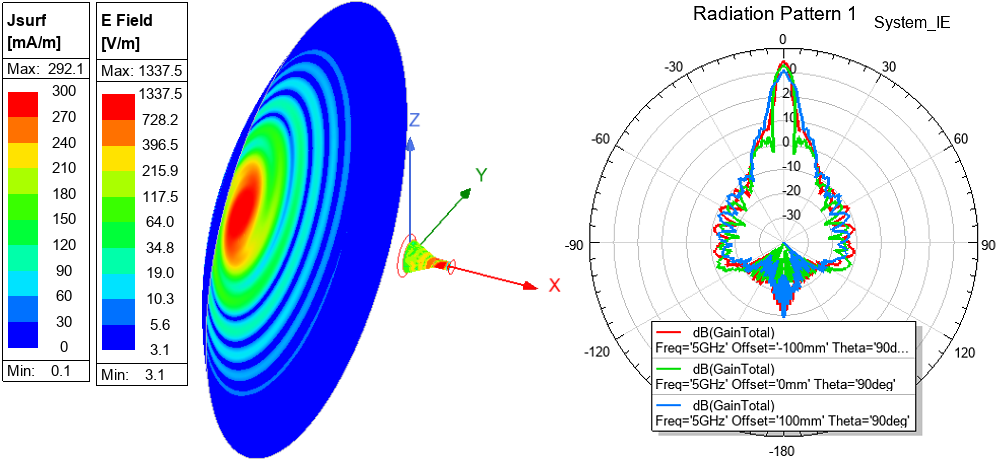
Radiation Pattern 1: Total Gain in dB for Offsets of -100, 0, and 100 mm
Realized Gain Plot 1: Realized Total Gain in dB at Nominal Offset (0 mm)
E-Field Magnitude Overlay (Horn)
Jsurf Magnitude Overlay (Dish)
Mesh Overlay (Dish)

You might want to switch to the default Isometric view for reviewing the fields overlays. Alternatively, rotate the Trimetric view slightly about the Z axis for a better view of the overlay on the concave dish surface. You can constrain rotation to be about the Z axis by pressing and holding the Z key while clicking and dragging using the middle mouse button. Move the mouse in a small arc around the center of the Modeler window. The model viewpoint will rotate about the selected axis the same number of degrees as the arc along which you drag the mouse.

The following image shows the Jsurf overlay on the Dish, the E-Field Overlay on Horn, and the Radiation Pattern plot for the System_IE design:

Parabolic dish model with E-Field and J-Surf overlays and Radiation pattern plot.

Double-click the predefined plots in the Program Manager's Results branches and the overlays in the Field Overlays branches to see them and to compare results between the System_IE and System_PO designs. For the field overlays, click and drag the E-Field legend and place it to the right of the Jsurf legend so that both overlays can be viewed simultaneously.