
NASA Almond Parametric
Abstract
This example is an HFSS design for reference results of a NASA almond monostatic RCS (radar cross section) analysis. The design is solved using the Integral Equation Method and is parameterized. A discrete sweep includes the adaptive solution frequency and two other frequencies. Two design are include, identical except for the polarization of the incident wave. The first design is for horizontal (HH) polarization, and the second, vertical (VV). The results match the reference publication[1] at 1.19, 7, and 9.92 Ghz for vertical and horizontal polarization.
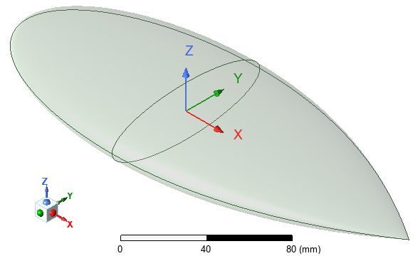
Figure 1: NASA Almond Geometry – Global Coordinate System
Simulation Time: (meshing, adaptive solution, and sweep in 2025 R1 using12 cores)
- HH Polarization: 4 minutes: 48 seconds, 1.54 GB max. memory per process
- VV Polarization: 4 minutes: 13 seconds, 1.48 GB max. memory per process
Model and Setup Details
The NASA almond is a solid constructed using two Equation Based Surfaces. Design variable "d" is defined to provide a scalable model.
Each surface is solidified using the following operations:
The two volumes are united.
Excitations:
- Plain Incident Wave – Spherical input format, used for monostatic RCS analysis (HFSS > Excitations > Assign > Incident Wave > Plane Wave). Polarization is horizontal for the first design (NASA_Almond_HH_Parametric) and is vertical for the second design (NASA_Almond_VV_Parametric).
Hybrid Region:
- IE Region, defined to solve using Full Wave BEM method (HFSS > Hybrid > Assign Hybrid > IE Region).
Mesh Operations: (Default initial mesh settings are used)
- Model Resolution (ModelResolution1): Length = 0.05 mm (HFSS > Mesh > Assign Mesh Operation > Model Resolution) – Set to avoid meshing excessively small details
- Surface Approximation (SurfApprox1): Settings are as shown in Figure 2 (HFSS > Mesh > Assign Mesh Operation > Surface Approximation) – Mainly used to control the mesh on true surface geometry (not segmented). Surface deviation controls the distance between the mesh and the true surface. Typically λ / 300 is chosen.
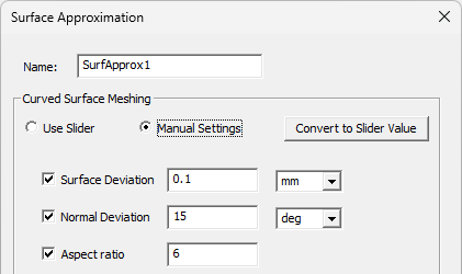
Figure 2: Surface Approximation Settings
The mesh can be imported into Hybrid (IE/SBR+) designs if there is an available source design and if no geometric changes are needed. For this example, you could choose to import the mesh from the HH design (horizontal polarization) into the VV design (vertical polarization). However, for this example the benefit of doing so would be minimal since adaptive meshing is limited to only two passes.
Setup: (9p92GHz)
- 9.92 GHz single adaptive solution frequency, default settings, Save Fields enabled
- Maximum Numper of Passes = 2
- Discrete sweep including three frequencies: 1.19, 7, and 9.92 GHz, Save Fields enabled
Based on the field accuracy , adaptive meshing will refine the most critical area. In this example, the current distribution is simple, and a single pass is sufficient to produce fair results. However, you can see that the results will slightly change from the first to the second pass. Generally speaking, the use of adaptive meshing is recommended for accurate and reliable results.
Postprocessing
After solving (Simulation > Analyze all), you can view different postprocessing results. Look in the Project Manager under Results and double-click on the different predefined reports. Each design also has to Jsurf overlays, one at 1.19 GHz, and one at 9.92 GHz. The first design (horizontal polarization) also includes a predefined mesh overlay. Figure 3 shows the available reports and overlays for the first design:
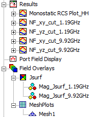
Figure 3: Predefined Reports and Field Overlays Listed in the Project Manager
Predefined Reports:
Figures 4 and 5 show the monostatic RCS results for all three frequencies that were solved and for the horizontal (HH) and vertical (VV) polarization, respectively:
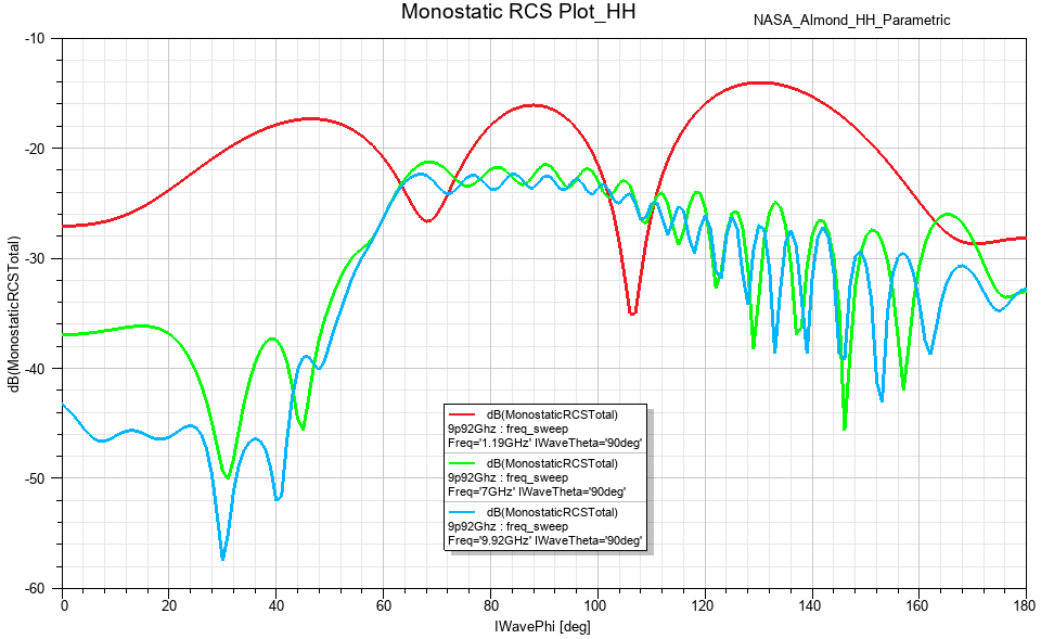
Figure 4: Total Monostatic RCS versus IWavePhi for Horizontal Polarization
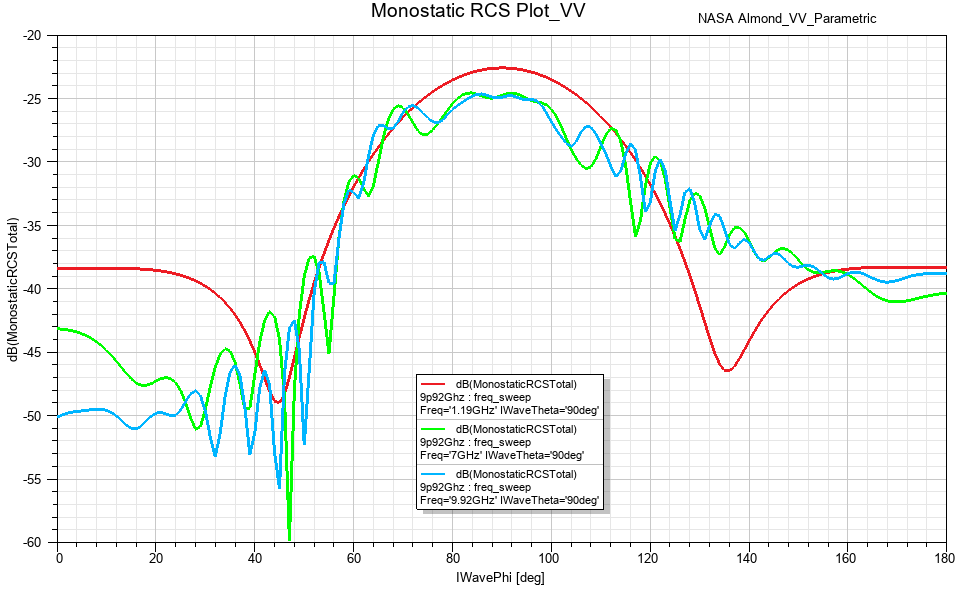
Figure 5: Total Monostatic RCS versus IWavePhi for Vertical Polarization
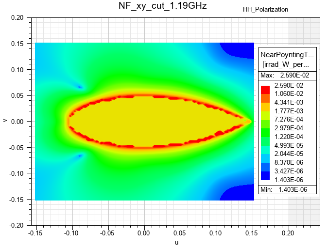
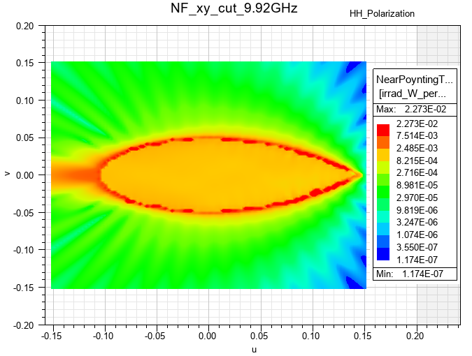
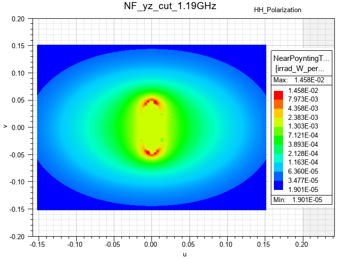
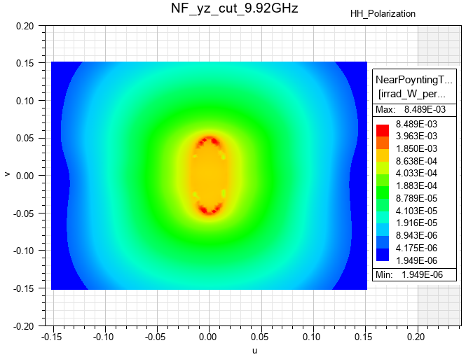
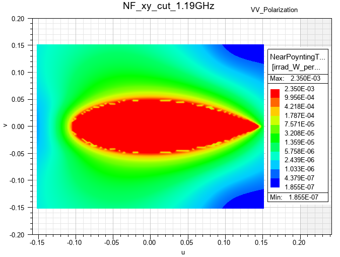
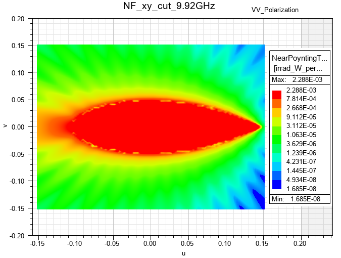
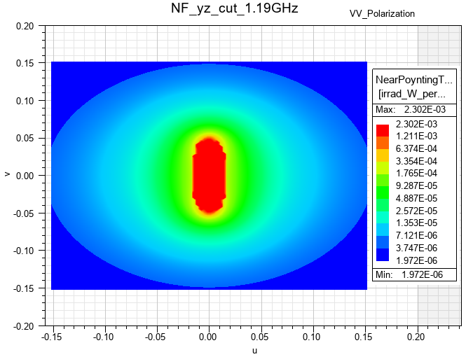
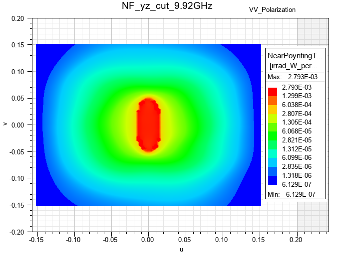
Figures 6 through 13 are near field contours at predefined rectangles that bisect the almond radar target. These figures include results at 1.19 and 9,92 GHz, horizontal and vertical polarization, and the near field radiation setups NF_xy_cut and NF_yz_cut. Results are also available at 7 GHz if you would like to modify one of the existing near field contour plots or add any plots.
In the eight contour plots that follow, you can observe nonzero fields within the conducting radar target body. The explanation is as follows:
- In the Finite Element Method (FEM), the solver directly computes the field solution within an air or vacuum region. However, within metallic bodies, the fields are set to zero instead of being computed.
- In the Integral Equation (IE) method (used for this example) or the Shooting and Bouncing Ray (SBR+) method, when creating a cut plane contour plot, the solution is derived from the current on the conducting body's surface. Inside metallic bodies, the total fields should ideally be zero, necessitating the scattered field to be exactly opposite to the incident field to achieve a total field of zero. Due to numerical inaccuracies, the field solution inside metals may be nonzero for IE and SBR+ methods, and it should be disregarded.
|
|
| Figure 6: Near Field Radiation Contours at NF_xy_cut – 1.19 GHz, Horizontal Polarization | Figure 7: Near Field Radiation Contours at NF_xy_cut – 9.92 GHz, Horizontal Polarization |
|
|
| Figure 8: Near Field Radiation Contours at NF_yz_cut – 1.19 GHz, Horizontal Polarization | Figure 9: Near Field Radiation Contours at NF_yz_cut – 9.92 GHz, Horizontal Polarization |
|
|
| Figure 10: Near Field Radiation Contours at NF_xy_cut – 1.19 GHz, Vertical Polarization | Figure 11: Near Field Radiation Contours at NF_xy_cut – 9.92 GHz, Vertical Polarization |
|
|
| Figure 12: Near Field Radiation Contours at NF_yz_cut – 1.19 GHz, Vertical Polarization | Figure 13: Near Field Radiation Contours at NF_yz_cut – 9.92 GHz, Vertical Polarization |
Mesh Overlay:
The first design includes a mesh overlay, which is shown in Figure 14. A mesh overlay was not added for the second design, since the model and setups are identical except for the incident wave polarization, and the element counts are the same.
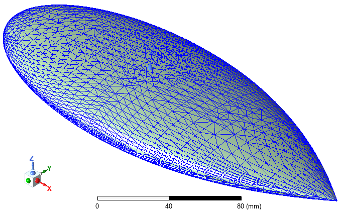
Figure 14: Mesh Overlay
Field Overlays:
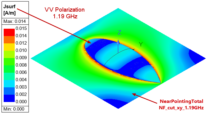
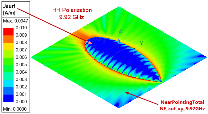
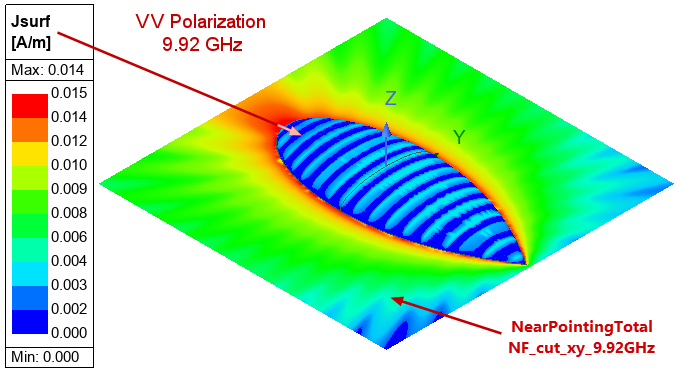
Each design has two predefined Jsurf magnitude overlays—one at 1.19 GHz and one at 9.92 GHz. See Figures 15 through 18. For each of these figures, the corresponding near field radiation contours are also displayed (HFSS > Fields > Plot Fields > Radiation Field). Additionally, fields are available at 7 GHz if you would like to modify one of the existing overlays or add a third one.
|
|
| Figure 15: Jsurf Overlay and XY Radiation Contours – 1.19 GHz, Horizontal Polarization | Figure 16: Jsurf Overlay and XY Radiation Contours – 1.19 GHz, Vertical Polarization |
|
|
| Figure 17: Jsurf Overlay and XY Radiation Contours – 9.92 GHz, Horizontal Polarization | Figure 18: Jsurf Overlay and XY Radiation Contours – 9.92 GHz, Vertical Polarization |
References
[1] "A. C. Woo, H. T. G. Wang, and M. J. Schuh, Benchmark Radar Targets for the Validation of Computational Electromagnetics Programs, IEEE Antennas and Propagation Magazine, vol. 35, no. 1, February 1993, pp. 84–89"