Differential Pair Stripline

The following figure shows a differential pair stripline design, where two copper traces are embedded in the substrate, which in turn is sandwiched between two ground conductors. Select GNDs on the project tree of the Project Manager window to highlight the ground planes assigned on the top and bottom faces of the stripline. These top and bottom ground planes are equipotential surfaces.

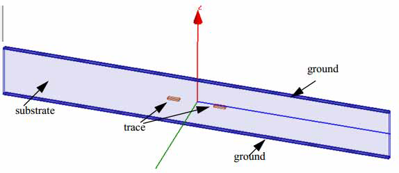
The intent of this design is to draw only minimal lengths of the differential traces containing the two conductors adjacent to each other (and the equipotential ground conductors) without explicitly drawing the actual length throughout the entire trace route. By using a post processing feature of Deembedding, transmission line characteristics can be calculated by moving the reference plane of the wave port to desired locations along the trace route, depending upon the specified value of the deembed distance. Such a design is an effective approach to simulate the actual model length. It saves simulation time and uses minimal computational resources.

Excitations

To see both excitations at the same time, right-click the Excitations option on the Project Manager window. Select List from the shortcut menu, and click the two wave ports listed in the Design List dialog box. The wave ports assigned in the model with the deembedded lengths appear highlighted in the design as shown in the following figure.

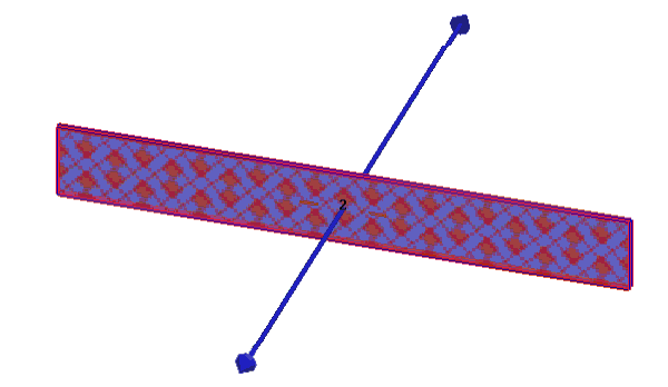
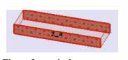
The deembed arrows point outwards from the structure since negative deembedding value of -(1in - ModelLength)/2 was specified for each wave port. The Deembed Distance value is set on the Post Processing tab of a wave port dialog box. The main purpose of such a design is to solve the model of minimal length and then, by deembedding outwards from the ports, to represent the actual length of the model. The terminals on a trace are shown in the following figure.

Solution Setup and HPC Analysis

Run this design at a solution frequency of 20 GHz. Since the design has a parametric sweep (with the trace edge-to-edge spacing defined by the variable S), it is a good choice for setting up HPC analysis. From the Solution Setup dialog box, click the button to open the HPC and Analysis window. Click Add to open the Analysis and Configuration window, where you can set the number of available cores to use for this design.

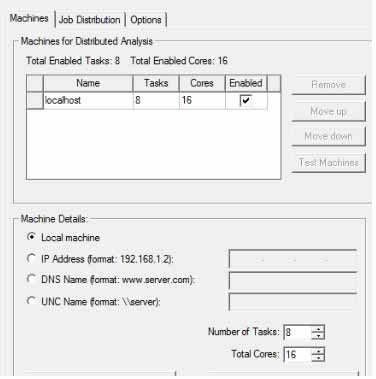
For example, in the figure above, 16 cores are available on the machine in which the design was simulated and number of tasks is 8. In such a setup, the sweep is run with 8 frequency points solved in parallel by using two cores of matrix multiprocessing for each frequency point. When such an analysis is executed on a single machine, the simulation is very efficient if the machine has enough shared memory to accommodate 8 simultaneous solves. Otherwise the analysis can be performed across multiple machines (that have HFSS installed in them) without requiring any additional HFSS license for each machine

While deembedding simplifies modeling long differential striplines and makes the solution process efficient, the HPC setup further accelerates the simulation process.

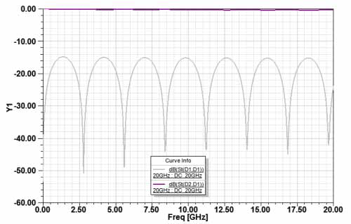
Results

The following figure shows the S-parameter plots for the stripline.