
Cylindrical Hyperlens
Abstract
Imaging applications are often presented with a difficult resolution barrier intrinsic to wave phenomena: the diffraction limit. While overcoming this limitation may seem impossible with a naive glance at Maxwell’s equations, in fact some further consideration shows it can be overcome through a variety of means. This example demonstrates one such method, a “hyperlens,” which has been realized at ultraviolet frequencies. This HFSS simulation predicts the hyperlens can resolve objects with separation of less than one-third the incident wavelength, well below the diffraction limit.
Simulation Time / RAM: (6-core machine with 64GB RAM in 2025 R1)
- Hyperlens Imaging: 1 minute: 34 seconds with 1.6 GB max. memory used per process
- No Hyperlens: 1 minute: 47 seconds with 1.33 GB max. memory used per process
Introduction
Imaging systems are essential technology in many industries, including medicine, semiconductors, defense, academic research, among others. While many of these systems are quite sophisticated, there are a few applications where optical imaging has yet to penetrate due to the diffraction limit hindering resolution performance.
For example, some sub-cellular processes of interest in medical research cannot be imaged in vivo due to their small size (much smaller than optical wavelengths) and the requirement for high vacuum inside electron microscope chambers. There are some existing sub-diffraction optical imaging methods, such as stimulated-emission-depletion microscopy, but the high optical power applied quickly leads to photobleaching and is limited to specific fluorophores.
Additionally, near-field scanning optical microscopy is a well-established commercial technology, but it requires relatively slow raster scanning of the sample, precluding it from real-time imaging.
Recent developments in electromagnetic metamaterials research have given us a few sub-diffraction imaging solutions at multiple portions of the spectrum [1-3]. One such technology of interest has been called the “hyperlens.” The hyperlens is constructed from a hyperbolic metamaterial, a special class of metamaterial that has dispersion relation described by a hyperboloid in three dimensions, in contrast to the usual ellipsoid. In addition to imaging, hyperlenses can also be applied to optical nanolithography and ultra-high-density optical data storage [2]. This example project shows one realization of a hyperlens from the literature which can achieve sub-diffraction resolution in the ultraviolet region.
Full-wave electromagnetic solvers like Ansys HFSS give engineers and researchers crucial information when designing and characterizing subwavelength electromagnetic devices, such as hyperlenses. This information includes parametric analysis, device optimization, and field plots.
Hyperbolic Metamaterials and Hyperlenses:
The dispersion relation for electromagnetic waves in spherical coordinates [4] is given by:
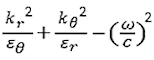
When εr = εθ > 0, the conventional diffraction limit constrains the resolution of any imaging process, since only waves with κθ≤ η(ω/c) will propagate. In other words, large spatial frequencies which carry the high-resolution image information, will not reach an imaging detector in the far-field. However, consider the case where:
εr < 0 and εθ> 0
In this case, the dispersion relation becomes a hyperboloid,
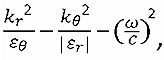
and arbitrarily large κθ can propagate. Such a medium, at optical frequencies, can be easily realized by modern nanofabrication methods, as in Refs. [4,5]. Fabricating the medium in a curved geometry then allows for magnification, so that as the large spatial frequency waves propagate through the medium, they also separate until they can be resolved by a conventional microscope after they exit the medium.
Model Construction and Setup Details
This example project shows simulation of a typical hyperlens imaging experiment similar to Ref. [4]. After setting up the HFSS project, the first step was to construct the layers of the hyperlens. The hyperlens consists of alternating pairs of metal and dielectric, in this case Ag and Al2O3. In principle, the hyperlens can be a truly three-dimensional device if fabricated in a hemispherical geometry. However, for this example it is sufficient to make it cylindrical and restrict the y-dimension with appropriate boundaries to save some computational resources. Also note that the experimental device in Ref. [4] is cylindrical, as we modeled here.
The layers were drawn by placing a series of concentric cylinders centered at the origin, subtracting each cylinder from the last one, then using a box command to subtract out the unwanted portion above the xy plane. The “object” being imaged is a Cr mask with two openings, separated by a subwavelength distance, on the inner radius of the hyperlens.
You can see the object history for the mask in the “Model > Solids > Cr_365nm” and "...Quartz_365nm" branches in the History Tree. After drawing the hyperlens and Cr mask, a box was then added to represent the quartz substrate. The hyperlens/mask structure was subtracted from the box and then the Separate Bodies command was used so that the portion near the center of the hyperlens could be deleted from the final structure.
A region was then added so that an incident beam and boundaries could be applied.
To give the model material properties, custom materials were defined using the permittivity values for a 365 nm wave-length given in Ref. [4]. Since the permittivity for Cr was not given, a value calculated from the commonly cited Lorentz-Drude model was used [6]. It is important to note that the time dependence convention adopted by HFSS requires that the imaginary part of ε and μ be negative for passive media.
Finally, because of the cylindrical geometry, the resulting “image” fields propagating away from the hyperlens have a cylindrical constant phase surface. Therefore, the image target, where we read out the fields, should be curved appropriately to mimic the phase compensation performed by a microscope objective. To do this, a curved line was added, away from the hyperlens, to later plot the fields along it.
Since this is essentially a two-dimensional problem, and the desired polarization determines that H should be oriented along y, Perfect H boundaries were applied to the ±Y faces of the model so that the computational domain can be reduced. Radiation boundaries were applied to the remaining outer faces.
To excite the model, a normally-incident Gaussian beam was added to the +Z face. Given that the operating wavelength for this device is 365 nm, the beam width was set so that it was not too small to show effects of diffraction but not larger than the total width of the model along the X direction. The final geometry is shown below. The two included designs are identical except for the absence of the hyperlens in the second deisgn.
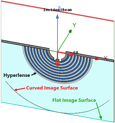
Figure 1: Design 1 – Hyperlens Imaging
The Curved Image "Surface" and Flat Image "Surface" objects are actually polylines. These non-model polylines are the specified geometry along which reported quantities are plotted. For the curved polyline, a dummy sheet object has also been created having a 10nm thickness (using the t_model variable). The original polyline was copied and given a thickness extending in a direction normal to the +Z axis and the arc itself (+/- Y in this case). The sheet is a model object, and its purpose is to force the mesh of the quartz boxes to conform to the target polyline. That is, solid element faces are generated along the sheet faces. This technique improves the smoothness of plot traces by eliminating the need to interpolate for results within the solid element interiors. The curved polyline, and therefore the sheet derived from it, is segmented to produce a consistant and regular mesh.
Before setting up the analysis, a length mesh operation was added to the hyperlens and Cr mask so that the fields inside the hyperlens can be well-resolved when later plotted. Since HFSS will adaptively mesh the model during analysis, this step is optional. However, since the fields inside the hyperlens layers are of some interest, it is nice to have a smooth picture of them when viewing the field overlay plots.
Since it is crucial for this model to accurately represent curved surfaces, it can be helpful to adjust some of the settings in the Initial Mesh Settings dialog box shown below. The relevant settings are the Apply curvilinear meshing to all curved surfaces check box and the Curved Surface Meshing slider:
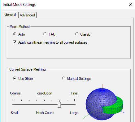
Figure 2: Initial Mesh Settings Dialog Box
It is worth noting that this slider will affect the number of elements in the model and, in turn, wil affect the memory requirements. However, in this case, the model is relatively small, using <1GB of memory for meshing, So there is little reason for concern.
The only remaining step was to add a solution setup with the frequency determined by the operating wavelength of 365 nm. The frequency can easily be determined from the wavelength by the relationship: f = c ⁄ λ.
Viewing Results with the Hyperlens
After analyzing the model, the results of interest can be easily extracted using the Results and Field Overlays branches of the Project Manager window. In this model, it is informative to view how the fields propagate through the hyperlens structure and into the Quartz substrate. Additionally, the resulting image is obviously of interest, so that we can determine if the Cr object is resolved. Fields overlays were plotted for both the magnetic field magnitude and the real part of the y-component of the magnetic field. The overlays have been assigned to the back face of the air region so that the curved image target polyline and its derived sheet object are visible from the front view while the overlay is displayed:
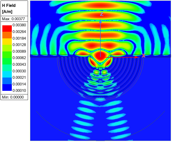
Figure 3: H Field Overlay – Hyperlens Imaging Design
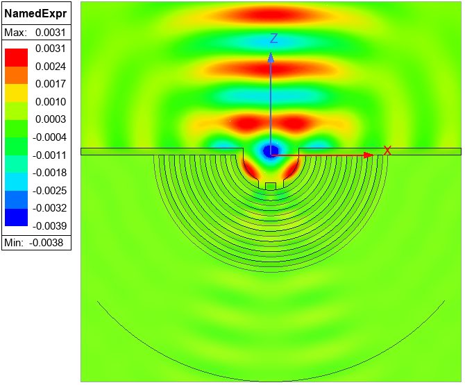
Figure 4: Real Part of Y-Component of H Field – Hyperlens Imaging Design
Animating this plot with respect to the phase gives interesting insight into how the waves propagate through the hyperlens.
The resulting complex E magnitude plotted along the previously defined curved image target is shown below. From this plot you can determine that the hyperlens effectively resolves an object having features with only 120 nm center-to-center separation, less than one third the incident wavelength and well below the diffraction limit.
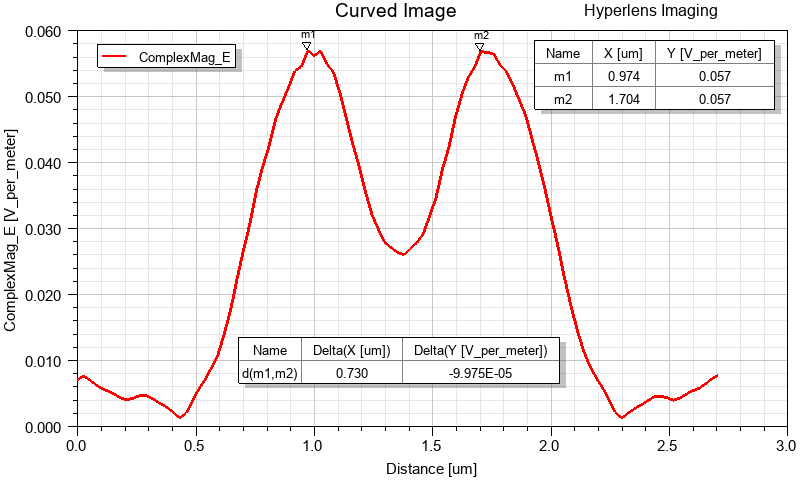
Figure 5: ComplexMag_E Plot – Hyperlens Imaging Design, Curved Image Target
Additionally, there is a predefined ComplexMagE plot for the flat image target:
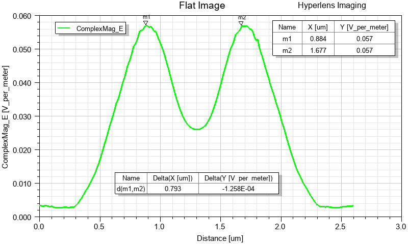
Figure 6: ComplexMag_E Plot – Hyperlens Imaging Design, Flat Image Target
Figure 6 clearly shows effective resolution of the small object, as also observed in the overlay in Figure 3 and the plot in Figure 5.
Comparing Results with and without the Hyperlens
A second model, without a hyperlens, is also included in the example project. It is used as a baseline comparison to illustrate the impact of the hyperlens design on field distribution and resolution. Below, the results with and without a hyperlens are compared side-by-side:
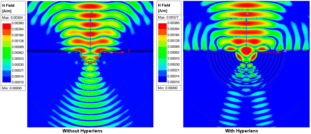
Figure 7: Comparison of H Fields without and with a Hyperlens
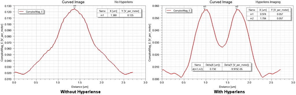
Figure 8: Comparison of ComplexMag_E Plots without and with a Hyperlens (Curved Image Target)
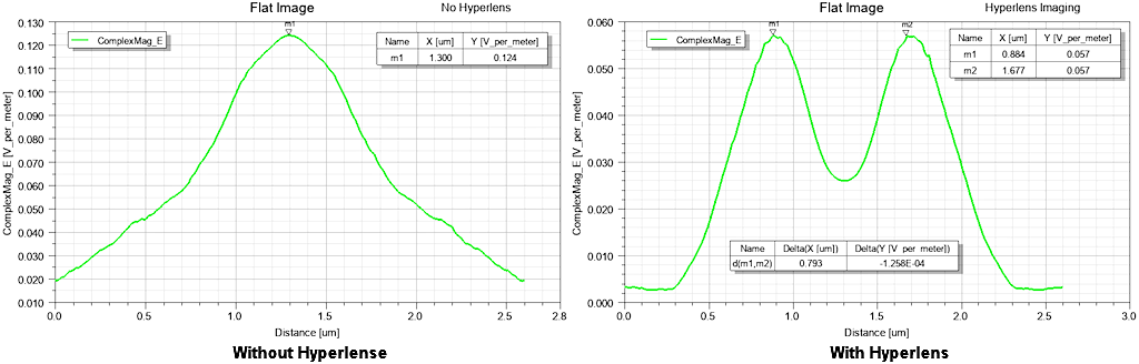
Figure 9: Comparison of ComplexMag_E Plots without and with a Hyperlens (Flat Image Target)
- The impact of a hyperlens is dramatically observed for both the Curved Image results (Figure 8) and the Flat Image results (Figure 9). In both cases, the two openings are seen as two peaks in the complex E magnitude traces. The plots from the No Hyperlens design show a single peak complex E magnitude at the center of the target, and the two separate openings are not detected.
- Note that the traces in Figure 8 (Cylindrical Images) are roughly symmetrical in shape and are centered at a Distance of approximately 1.35 um. Whereas, the traces in Figure 9 (Flat Images) are centered at a Distance of about 1.30 um. The flat target object starts at the far left edge of the model geometry and continues to the far right edge. The curved target object begins and ends at some distance inside the left and right extents of the geometry. Nonetheless, the curved object is longer than the straight one. Use the tool Modeler > Measure > Objects and click on each of the polylines that represent image surfaces to determine their lengths. The Flat_Image_Surface polyline object is 2600 nm long, and the Curved_Image_Surface object is about 2705 nm. The distances from the left endpoint of these objects to their midpoints differ by 52.5 nm (or about 0.052 um). The plots clearly reflect this distance variation.
References:
[1] X. Zhang and Z. Liu, Nat. Mater. 7(6), 435 (2008)
[2] D. Lu and Z. Liu, Nat. Commun. 3, 1205 (2012)
[3] W. Adams, M. Sadatgol, and D. Ö. Güney, AIP Adv. 6, 100701 (2016)
[4] H. Lee, Z. Liu, Y. Xiong, C. Sun, and X. Zhang, Opt. Express 15(24), 15886-15891 (2007)
[5] Z. Liu, H. Lee, Y. Xiong, C. Sun, and X. Zhang, Science 315(5819), 1686 (2007)
[6] A. Rakić, A. Djurišić, J. Elazar, and M. Majewski, Appl. Opt. 37, 5271-5283 (1998)