Connector - Terminal Example
Description - a simplified model of a four pin section of a connector. This is a driven terminal design.
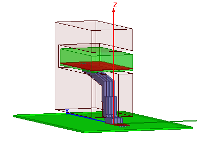
Model - the connector is configured with lumped ports on each end of the two inner pins. The two outer pins are each grounded at both ends. The boards are FR4 and the connector body is modified epoxy. A radiation boundary is applied to the surrounding airbox.
Setup - Driven Terminal Solution with adapt at 5 GHz. An interpolating sweep is also included that has an upper frequency of 5 GHz and uses DC extrapolation at the low end.
To view a port or boundary, select the desired item in the Project Tree. It is then highlighted in the Model window and the properties will be displayed in the Properties window. Selecting an object in the History tree will also display its properties.
HPC Analysis Setup
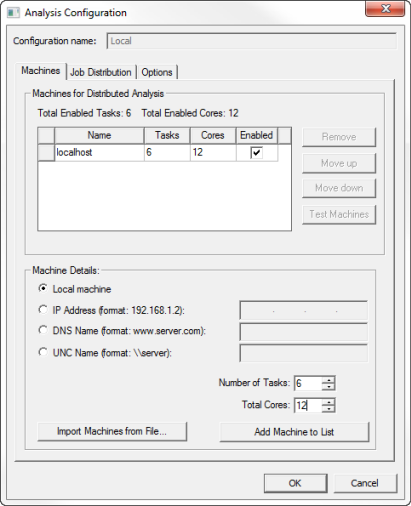
You can set an adapt frequency at 5 GHz with an interpolating frequency sweep from 0 to 5 GHz. Since several frequencies are being solved in this design, you can set up an HPC Analysis to distribute the frequencies resulting in efficient simulation.
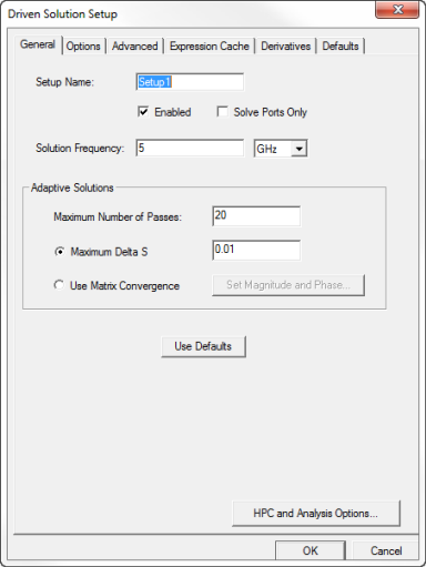
During the simulation, adaptive mesh refinement uses the Total Cores that are configured in the HPC setup, while the number of cores used to solve each frequency point is determined by Total Cores/Number of Tasks configured in the Analysis Configuration. On the Driven Solution Setup dialog box, if you click the HPC and Analysis Options button and click Add, you can set the Number of Tasks and the TotalCores on the Analysis Configuration window.
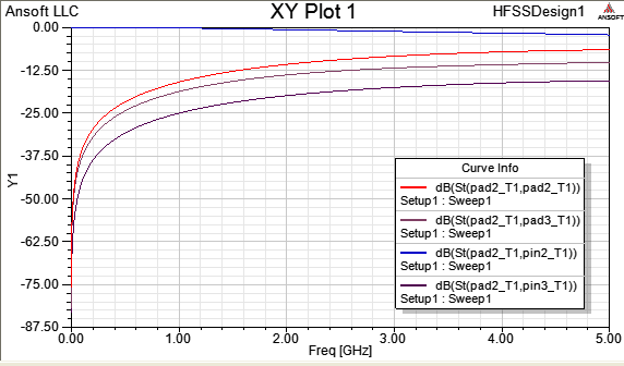
Connector Post Processing
After solving, you can view solution data by right-clicking on Setup1 and selecting Profile to display the Solution dialog. You also view the Solution tabs for Convergence, Matrix Data, and Mesh Statistics.
To view the S parameter plot show below, double-click on XY plot1 in the Project Tree under Results.