
Bandpass Filter
Abstract
This HFSS example shows a bandpass filter operating over a frequency range of 0.6–2.4 GHz.
The example project also has an associated getting started guide:
- Getting Started with HFSS: Bandpass Filter
Whereas the example model is fully set up, complete with predefined plots and overlays, and it is ready to solve, the getting started guide offers an alternative learning path. Follow it to walk through the process of drawing the waveguide geometry, assigning the excitations, setting up the analysis and frequency sweep, and evaluating the results.
Additionally, the getting started guide includes an HFSS Multipaction analysis, which is not included in the example model project. Refer to the getting started guide if interested in this feature.
Simulation Time/RAM: (meshing, adaptive solution, and frequency sweep; 16-core Intel i7 PC at 2.5 GHz; software version 2025 R1)
1 minute: 12 seconds, 635 MB max. memory per process
The project file, Bandpass_Filter.aedt, is located in the ...Examples\HFSS\RF Microwave subfolder of the program installation path.
Description
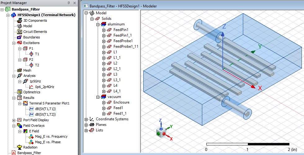
This HFSS example model is an interdigital bandpass filter with a bandwidth of 1 GHz. The conductors are surrounded by a vacuum enclosure, and the filter is fed by a 50-ohm coaxial transmission line.
While radio frequencies behave nearly identically between air and vacuum regions, the multipactor effect only occurs in a vacuum. For this reason, vacuum is needed for the getting started guide's multipaction analysis, and the example model's construction and materials are kept consistent.
Analysis Setup:
The analysis setup and frequency sweep are predefined, as follows:
- Analysis Setup: Name = 1p5GHz ("p" is used because decimal points are not permitted in setup names); Adaptive solution frequency = 1.5 GHz; Automatic selection of Direct or Iterative solver is selected.
- Sweep: Name = 0p6_2p4GHz; Type = Fast; Distribution = Linear Count; Start = 0.6 GHz; Stop = 2.4 GHz; Points = 451
HPC Settings:
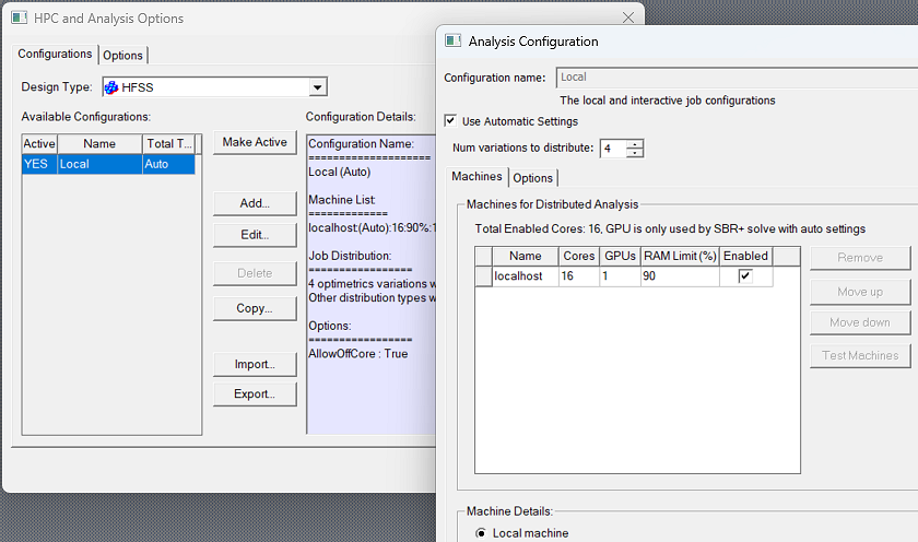
You can set up a High-Performance Computing (HPC) analysis to distribute the sweep frequencies (that is, to solve multiple frequencies in parallel) resulting in a faster simulation. The number of cores used to solve each frequency point is determined by Total Cores/Number of Tasks configured in the Analysis Configuration. Additionally, adaptive mesh refinement uses the Total Cores you specify in the HPC setup. You can access these settings from Tools > Options > HPC and Analysis Options and then by clicking the Edit button on the HPC and Analysis Options window to see the configuration for this design.
To view a port definition, select the desired excitation in the Project Manager. It is then highlighted in the Modeler window, and the settings are displayed in the docked Properties window. Selecting an object in the History tree also displays its properties.
To solve the simulation, right-click on 1p5GHz, under Analysis in the Project Manager and choose Analyze from the shortcut menu.
Postprocessing
After solving, you can view the solution data by right-clicking 1p5GHz (under Analysis in the Project Manager) and selecting Profile to display the Solutions dialog box. In addition to the Profile tab, you also view the Convergence, Matrix Data, and Mesh Statistics tabs.
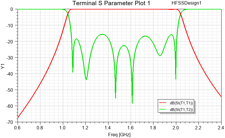
To view an S parameter plot, expand the Results branch of the Project Manager and double-click Terminal S Parameter Plot 1. You can add markers to the XY plot by right-clicking in the plot window and choosing Marker > Add Marker.
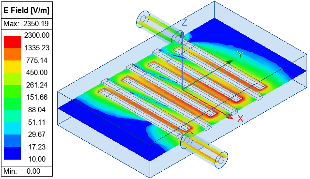
Two electromagnetic field overlays are predefined for this filter and are listed under Field Overlays in the Project Manager. For both overlays, the scale is logarithmic, and range limits have been defined to produce a good range of color contours for all frequencies and phases when the overlay is animated.
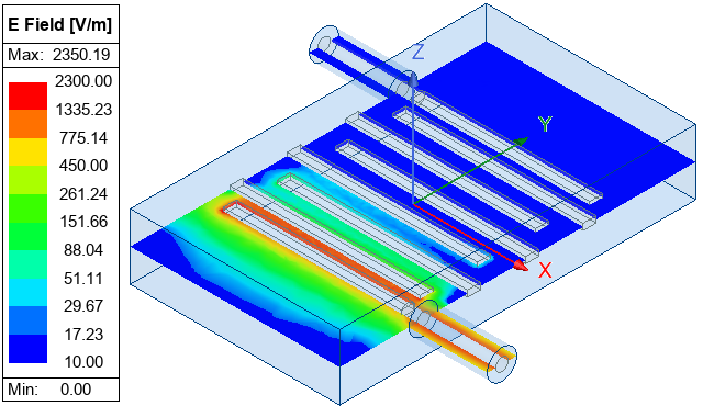
The first overlay, E Field > Mag_E vs. Frequency, is intended to show how the field varies over the swept frequency range. It shows the field along the global XY plane, which is the horizontal midplane of the model. The initial frequency is 600 MHz, which is outside of the pass-through bandwidth of the filter. Therefore, the signal is blocked from reaching the output port. The phase angle is zero degrees:
The second overlay, E Field > Mag_E vs. Phase, is intended to show how the field varies with phase angle. It also shows the field along the global XY plane. This overlay is at the adaptive frequency of 1.5 GHz, well within the bandpass frequency range of the filter, and is initially at a 0-degrees phase angle:
Two animation setups are predefined:
- Frequency Animation (Swept variable Freq): Use to animate overlay Mag_E vs. Frequency
- Phase Animation (Swept variable Phase): Use to animate overlay Mag_E vs. Phase
The following animation is the E Field versus phase at the adaptive solution frequency of 1.5 GHz:
The following animation is the E Field versus frequency:
For the frequency animation, notice that the electromagnetic field only reaches the output port for the inclusive frequency range of 1.0 to 2.1 GHz.