Guidelines for Sampling Frequency Responses

State-space fitting can deal with quite significant gaps between samples, especially if each of the given samples can be predicted very accurately by a low-order (compared to the number of samples) model. But if the samples are somewhat noisy or are sampled from a system that has a large number of poles, a fitting algorithm might not produce an accurate, passive, and smooth fit. Ideally, samples should be such that no resonance is missed, and the data should vary fairly smoothly from one sample to the next. One rule of thumb is that the difference between a spline interpolation of the data and a linear interpolation of the data should be fairly small, say no more than 0.1-0.2 for S-parameters.

Figure: Adequate and inadequate sampling of a resonance, judged by the difference between linear and spline interpolations.

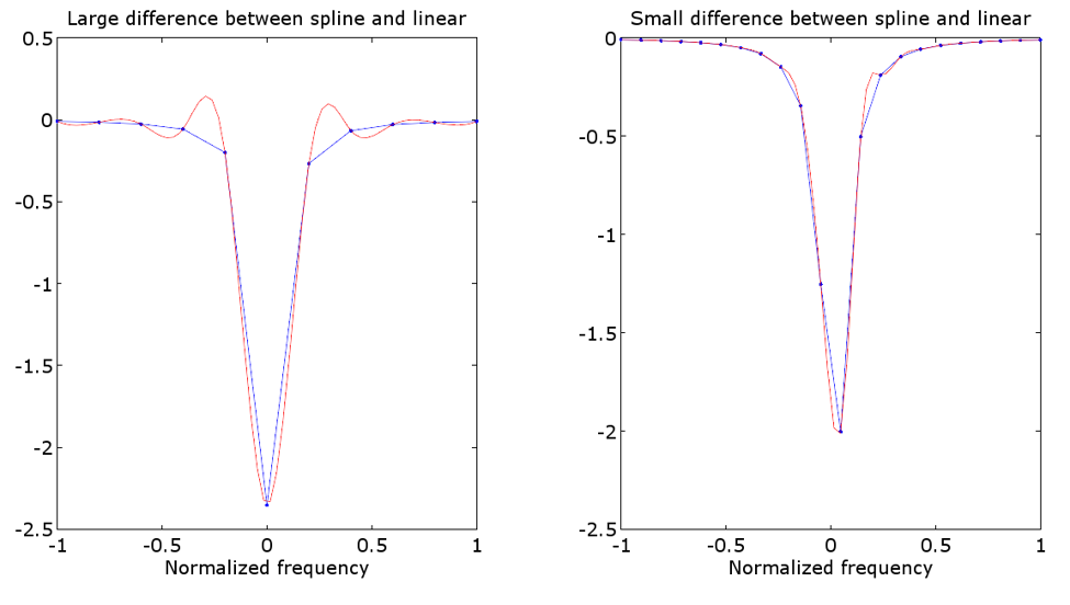
The sample frequencies should start as low as possible, preferably at DC, and end only once high-frequency losses become apparent, so the 2-norm of the S-parameter matrix begins to taper off. For systems with very small losses, this might be too high for practical simulations or measurements. The fitter should be able to handle such cases, in which the losses are very small throughout the sampling band, but they are challenging. The reason these cases are difficult is that the state-space model can in principle assume any values in these gaps or out of band. While the FastFit algorithm controls the magnitude of the fit in these gaps (and out of band), significant passivity violations may still occur. Then, when passivity is enforced, removing these passivity violations entails a significant perturbation of the fit, which results in significant errors w.r.t to the data. If it is not practical to sample up to a frequency in which losses become apparent, then at the very least the highest frequency should be above the highest frequency of the excitations that is used in the time-domain simulation.