Using the Device Characterization Wizard for a Thyristor

The following procedures use an ABB device as an example. The process is similar for other manufacturers’ devices.

1. In the Component Information [1/9] dialog box, enter the component name, and define the manufacturer's measurement criteria. If thermal or depletion capacitance characteristics are available, clear the Hide & Disable option in this page.

2. The Nominal Working Point Values [2/9]

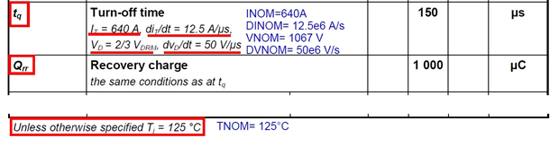
• Nominal Values – This section sets nominal values at the device’s working point. These values should be the test conditions of Qrr or Tq on the manufacturer's data sheet. The test condition is later used during model extraction, when model parameters are optimized to match the model’s characteristics in the same test condition with datasheet values. When Qrr data is available for multiple temperatures, select the Tj nom for which you have the on-state characteristics in the plot section.

I leak_r and I leak_bl are the leakage current in reverse and blocking mode. Use default values if not known.

• Device & Circuit Values – If specified by the datasheet, input the snubber and stray inductance values; otherwise, use 0, then snubber parameters will calculate during extraction.

Click Next to continue.

3. The Device and Limit Values [3/9] dialog box.

• Trigger Definition

Only the digital trigger option is available for now. Input parameters set the trigger condition of the model; values can be found in the datasheet.

V trig - Gate trigger voltage, model turns on when gate voltage is above this value.

I hold - Holding current.

Td_q - Gate turn-on delay time.

Tq - Circuit commutated turn-off time.

• Limit Values

Use the default breakthrough characteristics, as the data is rarely available in a datasheet.

4. Use the On-State Characteristic [4/9] dialog box to parameterize the on-state current characteristics of the thyristor. At least one set of input data at nominal temperature (input in dialog box [2/9]) is required. A second set of data at a different temperature is preferred in order to characterize temperature dependency parameters.

Choose one of the two ways to input: Use Data Table or Use Equation Coefficients. If both types of data are available, choose the type with data at both nominal temperature and a different temperature.

• Use Equation Coefficients - If provided, these coefficients are usually in a table of A, B, C, D parameters.

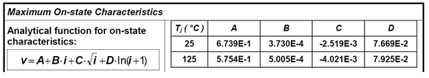
1. From the drop-down list of analytical functions, select one that matches the equation specified in data sheet.

2. Input the value of A, B, C and D, and set the temperature.

3. In the Fitting Range panel, define the effective iT range of the analytical function. It is usually provided with the function, as shown below.

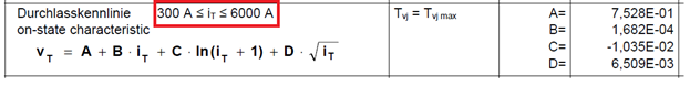
You can also look for range of iT in the on-state characteristics figure. For example, in the plot below, the effective range of iT is roughly 200A to 3500A. Note that the analytical function is usually not valid close to iT=0A, so it is important to define the lower range of fitting.

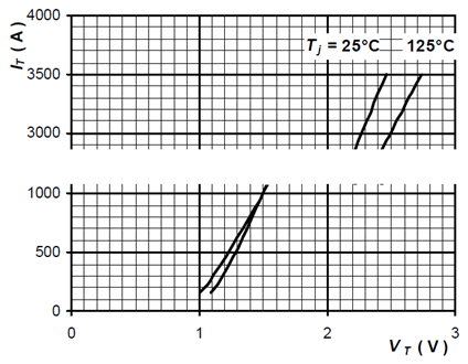
If none of the above information is available in regards to effective range, click the two arrows to let the wizard estimate proper current range.

4. To add a characteristic at a different temperature, click Add new characteristic in the top right, then repeat steps a, b, and c.

Proceed to Fitting the On-State Characteristic.

• Use Data Table - Sample data from the on-state characteristics plots.

Enter the data with SheetScan. To do so, click Load characteristics from Dataset Manager above the table and click SheetScan. Load the graphs in the graphic files captured from the manufacturer data sheet using Picture > Load.

1. Select a coordinate system (Coordinate System > New) and define it on the plot. To do so, you must select three points. Typically, you should use the bottom-right, bottom-left and top-right points of the plot grid. Click Point1, Point2 and Point3, and select the corresponding points on the graph. Enter the corresponding X-values and Y-values for these points (read from the plot’s X-axis and Y-axis labels) in the table, and click OK to finish defining the coordinate system.
2. To define the first characteristic, select Curve > New, and give names to the X-axis and Y-axis in the Curve Settings dialog box. Click OK when finished.
3. Make sure to note the temperature given on the plot. Then select several points on the curve starting with the lowest X-value. Pick at least four points. When done, click File > Export and click Dataset in the resulting Save dialog box.
4. If a plot at a different temperature is available, repeat steps a, b, and c to record additional data.
5. When finished, click File > Exit to exit SheetScan, saving the scan setup information if desired.
6. In the Datasets dialog box, select the data you want to use at the nominal temperature and click Done. The data is transferred to the Characteristic Data table in the On-State Characteristic [4/9] dialog box. Make sure to enter the correct temperature values which you recorded during the SheetScan measurements.
7. If you also recorded plot data for a different temperature, click Add new characteristic in the top right, then click Load characteristics from Dataset Manager above the table to load the additional data.
   • Fitting the On-State Characteristic
   1. In the Fitting Characteristic Order panel of either tab for input data, select the Nominal Temperature, which is the same as Inom input in [2/9].
   2. If you added a second set of data for a different temperature, you can select the temperature for the Different Temperature field, or select Not Used, if data is available only for one temperature. If Not Used, the model’s static parameters for temperature dependency will be 0.
   3. Click Start Fitting to fit the characteristics, and examine the resulting plot to check the match of the fit. Click Next to continue.

5. Use the Thyristor Thermal Model [5/9] dialog box to parameterize the thermal impedance of the thyristor. If no thermal data is available, or thermal behavior is not interested in simulation, select No Data Available or Isothermal to skip this step. Otherwise, if this dialog box is not displayed, make sure Hide & Disable Thermal Characteristics in [1/9] is cleared. To fit thermal characteristics, do one of the following:

• Use Fraction Coefficients - If the data sheet provides extracted values for Ri and Taui, enter these value pairs in the Thermal Coefficients table. Click Add new point on the top right of the data table to add orders as provided in data sheet. Click Start Fitting, check the plot, and click Next to continue.

• Use Transient Thermal Impedance - If the data sheet does not provide extracted values for ri and ti, select Use Transient Thermal Impedance and enter the plot data for the thermal characteristics using SheetScan per the instructions given in step 4. The plot shows the impedance as a function of time. Make sure to adjust the scale of the coordinate system in SheetScan to logarithmic if needed.

Click Start Fitting, check the plot, and click Next to continue.

6. Use the Depletion Capacitance Characteristics [6/9] dialog box to parameterize the thyristor junction capacitance vs. the reverse voltage. In most cases where such data is not available, skip this step.

If the data sheet provides junction capacitance vs. reverse voltage characteristics, make sure Hide & Disable Depletion Capacitance Characteristics in [1/9] is cleared, so this dialog box displays. In dialog box [6/9], clear Disable Cv Characteristics, and enter the junction capacitance data with SheetScan. Select Start Fitting to start the fit, and examine the plot to check the match of the fit. Click Next to continue.

7. Use the Dynamic Model Input [7/9] dialog box to parameterize the dynamic characteristics of the thyristor. You can select to fit for the reverse recovery measurements. The nominal point has to be fit, so some data at this working condition must be available.

By default, reverse recovery charge Qrr and reverse recovery time Trr are the displayed goals to fit. If only Qrr is available in the datasheet, clear the other goals to disable them. If other measurements are available in the datasheet but not displayed in the wizard, for example, reverse recovery peak current Irm, click Advanced Settings and go to the Model & Goal Settings tab to add fitting goals by checking them in the Select Goals to Display panel.

Turn-off time Tq does not play a role in dynamic extraction, since the thyristor model has only digital ignition. Tq is modeled as a timer set directly by parameter TQ, which is input in dialog box [3/9]. Note that Tq is not equivalent to reverse recovery time Trr: it is usually much longer (3-5 times) than Trr.

The Advanced Settings button allows for more control over the characterization process. Some parameters are important for extraction to succeed. See the Advanced Settings documentation for more information.

1. Click Measurement to open the Measurement Data dialog box and make sure the settings correspond to the ones for the manufacturer of the device being characterized.
2. If data is available at different temperature, add it to the dT row.
3. If data is available at a different value of current I_d, add the lower value of current to the nI row and the higher value of current to the pI row.
4. Click Extraction to start the fit, then click Next to continue.

Advanced Settings

• H_MIN – Minimum step width during extraction. Suggested value: Trr/1000. H_MIN should be small enough to have good resolution of reverse recovery waveform. Suggested H_MIN during extraction is smaller than what should be used in the final simulation because during extraction, dynamic parameters are being tuned and reverse recovery waveform is changing and could be a much smaller Trr measurement than the goal value. The H_MIN setting here should still give enough resolution in such cases.
• H_MAX – Maximum step width during extraction. Suggested value: 100*H_MIN.
• PERIOD – Switching period during extraction. Suggested value: 3*Tq.
• H_ON - Reverse recovery signal acquisition time, should be set to 2-5 times of Trr. This parameter is crucial for extraction success.

• H_OFF - Not used.

• The parameter extraction process uses three optimization routines to determine values for the dynamic device parameters. Thyristor extraction uses the first routine, which is an iterative loop that uses a 1D search method to progressively refine its approximation. LOOPS_A sets the number of loops in this routine; the default value is usually sufficient. MASKPAR_A contains the names of the optimization parameters to reach a good convergence, and the default setting enables both parameters, which is usually good. RESORD_A sets how the residue is defined: 0 (zero) for the maximum error, 1 for the average error, and 2 for the root mean square error. RESTOL_A defines the value under which the residue must get to leave the loop with a good solution.
• The second and the third loops (B and C) use a Jacobian matrix method. These loops are usually not used for thyristor extraction.

8. Use the Dynamic Parameter Validation [8/9] dialog box to validate the dynamic extraction. The actual reverse recovery characteristics for the parameterized device are simulated and measured. Enable the conditions that need to be checked and click Validate. Click Next to continue.
9. Use the Model Parameters [9/9] dialog box to browse the extracted parameters.

1. To generate an .sml file of the model, click Create SML.
2. To place a characterized device in the Twin Builder project, click Place Component and click Finish.
3. To generate a test circuit using the characterized device, click Testcircuit and click Finish.