Advanced Settings for Characterizing a Basic Dynamic IGBT

Click Adv. Settingsin the Dynamic Model Input [10/12] dialog box to access the advanced settings of basic dynamic IGBT characterization. There are two tabs: Extraction Settings and Model & Goal Settings.

Extraction Settings

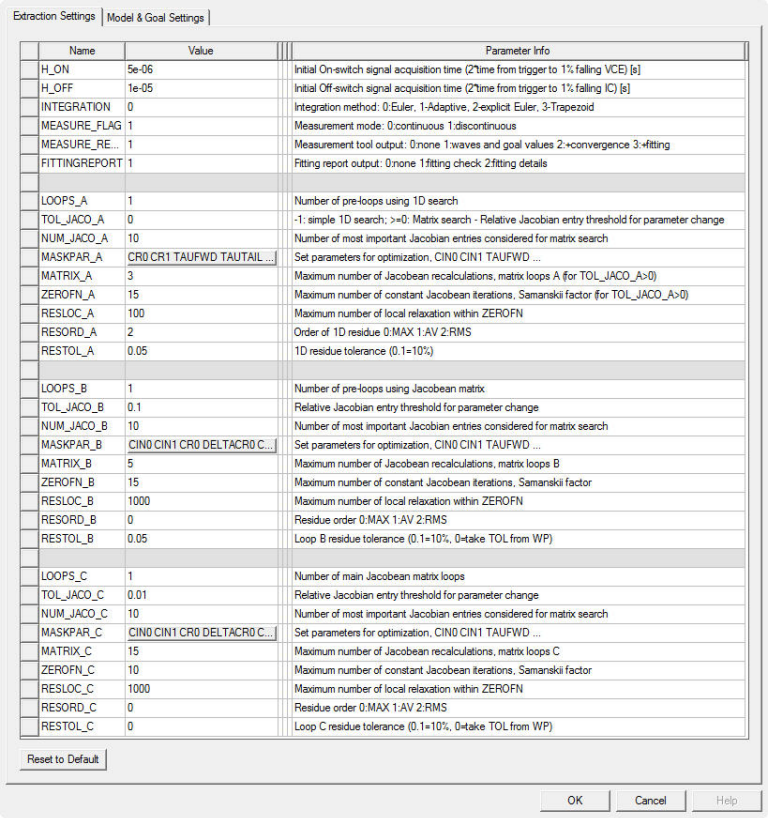
Advanced Parameter Setting Dialog Box

These settings give you more control over the characterization process, but it should not be necessary to change them for most devices.

Parameter

Information

H_ON and H_OFF

Before preprocessing and interpolation of the on/off switch wave forms, a series of simulated data points must be stored temporarily. These parameters set the acquisition time for the data points. This time interval setting limits the amount of acquired data and must fit to the longest possible time constants at the on/off switch together with a remaining time buffer to allow the Jacobean entry calculation which sweeps every parameter in a wide range. The sensitivity analysis for the 1D search in loop A varies actual parameters from p-25% ... p+50% and the Jacobean-based method does a parameter variation in the range p-10% ... p+10%. This is repeated several times to calculate either the actual best fitting single parameter or a parameter to goal sensitivity coefficient. Thus, the transient wave form duration will vary in a wide range.

H_ON and H_OFF are the initial settings for the On-switch and OFF-switch signal acquisition times. The actual Hon and Hoff values change during the characterization. Hon and Hoff derive from the measured switching times and length of the reverse recovery. 5x…10x of the On-switch/reverse recovery time should be a good value. For SiC devices the values should be much smaller than for Si devices. If the initial values are not good, the extraction process will not determine the sensitivity of parameter changes to the output signal and the extraction will not start to converge. You can observe the convergence of the extraction on the Fitting info page and adjust the initial values for H_ON and H_OFF if necessary.

INTEGRATION

Integration method (0 - best for switching devices).

MEASURE_FLAG

Measurement mode (1 – allows for stop of measurement cycles as soon as good result is reached).

MEASURE_REPORT

Measurement tool output (should stay 1).

FITTINGREPORT

Fitting report output (should remain set to 1).

LOOPS_A, LOOPS_B, and LOOPS_C

Approaching the optimal parameter set is an iterative procedure. This iteration is split into three sequenced loops: A, B and C. Each of the sequences can be repeated any number of times according to LOOPS_x. This is especially helpful in the case of loop A, which is a predefined sequence of one dimensional parameter sweeps. In some special cases, an increased number LOOPS_A can result in much better initial parameter values before starting the Newton-Raphson-based matrix loops B and C.
But the repeated 1D parameter sweep will take time and a global convergence is not guaranteed. In most cases the initial values calculated internally from the nominal conditions are good enough to start loop B immediately without time-consuming loop A.

Default values are LOOPS_A:=0, LOOPS_B:=1, and LOOPS_C:=1.

MASK_PAR_A

This is a list of dynamic model parameters which take part in the 1D parameter sweep sequence. The input is interpreted as a parameter mask for parameter selection during the characterization. Parameter names in bold mark the values included by default.

Parameter	Observed impact to goals
CIN0	Eon, Eoff
CIN1	Ton
TAUS	Toff
CR0	Ton, Toff
CR1	Ton, Toff
TAUFWD	Eon
DAMPING	Eoff
RG	Ton
DELTATAIL	Toff, Eoff
TAUTAIL	Toff, Eoff
L_EXTERN	Eon, Eoff

A repeated application of loop A helps to find a good initial parameter guess for the following Newton-Raphson-based loops B and C.

The above table also shows the most likely parameter-to-goal impact which is useful in case of manual parameter optimization.

MASK_PAR_B and MASK_PAR_C

Lists of dynamic model parameters which take part in the Newton-Raphson-based parameter optimization by error minimization. The following parameters are recognized. The parameters included by default are in bold letters.

Parameter	Meaning
CIN0 CIN1	The constant input capacitances are split into two values which take effect either at the on-switch edge (1) or at the off-switch edge (0). Generally, the input capacitance is expected to be a constant value but depends really on the state of the MOSFET channel and the applied GS- and DS voltages, which is highly complicated. By splitting CIN into two independent parts, the parameter optimization gets less complicated. The transition from CIN0 to CIN1 takes place at the trigger moment before any change by transition. Internally the charge balance is preserved to avoid unexpected current injection. CIN0 and CIN1 should change during the optimization in a similar range and stay much larger than the corresponding feedback capacitance CR0 and CR1 to ensure stable simulation results. If one of CIN0 and CIN1 changes greatly, especially toward smaller values, then this CINx should be deleted from the list before restarting the extraction. In some cases the whole characterization becomes unstable because CIN0+CIN1 gets much too small compared to CR0+CR1. In this case, you can exclude CIN0 and CIN1 ; the solution must then be found using the initial CIN values. Normally you can take the data sheet values as initial values. If CIN is not available, input zero so the initial value can be derived from the nominal values.
CR0 CR1	Feedback capacitance CR is also split into off(0) and on(1) parts (see CIN) to reach a better match with the optimization targets. It is selectable if CR is a constant or a voltage dependent value, under Model & Goal Settings. The data sheet values can be taken as initial values. If CR is not available, set zero for the initial value calculation derived from the nominal values (see CIN). In general the initial input CIN:=0 and CR:=0 will work and result in a parameter optimum. But to save time a good initial guess for CIN and CR is recommended.
DELTACR0 DELTACR1	For a rough calculation or to find a better initial guess DELTACR values can be excluded. Excluding parameters enhances the optimization speed. For example, you can exclude DELTACRx in loops A and B if the refinement loop C will follow. If DELTACRs are enabled or part of the parameter list, more accurate optimization results for different working points are expected. More parameters, which must have non-vanishing impact to at least one goal value, result in a larger freedom of the optimization problem and faster convergence. However, there is no clear rule if a maximum number of free parameters will accelerate simulation and increase the accuracy. The most important rule is that the parameter impacts-to-goal values should have minimum correlation. This information is not available before the optimization run, so sometimes trial and error is a useful way to find an optimum solution.
TAUFD	This parameter directly influences the amount of excess charge storage of the active freewheeling diode. Thus, the impact can be seen in the on switch current overshoot area. Eon of pn- junction devices strongly depend on TAUFD setting – if a freewheeling diode is used and really active at the considered switching edge. Resistive switching time test circuits don't show this effect. Thus, the parameter TAUFD becomes meaningless and must be excluded from the parameter list. If in general a meaningless parameter or a parameter having very low impact to any selected goal value takes part in the optimization, it takes much longer and the convergence path may deteriorate. Shottky junction devices or modules having a Shottky freewheeling diode anti-parallel to the semiconductor switch don't store excess carriers in the junction region. You can use at least a minimum TAUFD value to be able to adjust the capacitive reverse recovery.
SF	The larger the soft factor SF, the smaller the current overshoot gets and the longer the reverse recovery time t_RR is. In most cases SF can stay at default. If the optimization for loss energies and delay times together becomes difficult or the process of optimization takes much more time than expected, the inclusion of SF may solve the problem. The optimization result should be in the range 1 … 7.
TAUTAIL DELTATAIL	Both parameters are intended to control the current tail effect due to excess carrier storage in the active switching device at the off-switch edge. Assuming the current tail as a falling exponential function starting at the off-switch trigger moment, the current duration can be controlled by the time constant at 1/e = 36.8% of the starting value. Thus, TAUTAIL must be in the same range as the off switch delay Toff and the storage time TAUS. Much too large TAUTAIL problems with H_OFF arise and much too small initial values will practically exclude TAUTAIL from the parameter optimization because of negligible impact. DELTATAIL sets the starting value compared to the load current just before the off-switch. It can be even larger than 1 to reshape the off-switch edge and thus to control the off-switch energy in any case. You should include both parameters in the list for any material and technology.
RG	RG is the internal gate resistance due to the spreading resistance of poly silicon. Sometimes a separate resistor is added to limit the input current at the switching edges. It impacts all goal values because it controls the charging and discharging speed. If external gate resistances given in the data sheet RG should be set to 20% of (RG_ON + RG_OFF)/2. RG is treated as a free parameter to find the best trade-off between all goal values. RG should be part of the characterization in all cases.
TAUS	This parameter has direct feed through to the off-switch delay time. It controls the miller level duration and thus the off-switch storage time which is the main part of the off-switch delay time Toff. All devices must include this parameter.
DAMPING	Calculated from the stray inductance and the feedback (Miller) capacitance, each component gets an internal RC- snubber parallel to the output terminals. For a rough characterization, set DAMPING:=1 and leave it untouched. DAMPING is useful for solution refinement especially in loop C.
L_EXTERN	If the external stray inductance of the test circuit is not known (as in most cases), it is possible to include this value in the parameter optimization. L_EXTERN influences the distribution of the total switching energy across the on and off switch edge. If L_EXTERN is included, the convergence speed improves. By default, a fix value of 2nH is assumed instead if changing L_EXTERN.
LAUX	The value of the inner emitter inductance has impact to di/dt and dv/dt. This parameter is especially useful to slow down the voltage rise at switch off. For parallel connected devices it controls the amount of ringing.

NUM_JACO_A, NUM_JACO_B, and
NUM_JACO_C

This parameter defines which entries from the sensitivity matrix are considered for the matrix search:

-1: largest column, 0: apply threshold >0: this number of largest entries

For Loops_A when using a simple 1D search, this parameter is ignored.

TOL_JACO_A,
TOL_JACO_B, and TOL_JACO_C

This parameter defines the relative threshold for Jacobian entries to be used in the matrix search (when NUM_JACO_x = 0).

For LOOPS_A it can be set to -1 which will switch LOOPS_A to simple 1D search.

RESORD_A, RESORD_B, and RESORD_C

This is the order of the residual. The number range is 0 .. 2:

0 – The maximum error is the residual value (the error number).

1 – Absolute error average.

2 – Root mean square error value. If the initial parameter set is far off the optimum solution (for example, RESORD_A) this parameter should be 2. toward the optimal solution, to achieve a certain error limit (for example, RESORD_C) this parameter should be 0.

RESTOL_A, RESTOL_B, and RESTOL_C

Desired accuracy of the residual according to the RESORD setting. To quickly move the model parameters toward the optimum, the tolerance can be set as large as 0.2 = 20%. The number of necessary loops A, B and C will decrease strongly. Use the final accuracy only in the last main loop (usually loop C).

Relaxing the accuracy can result in a noticeable reduction of simulation time.

MATRIX_A,
MATRIX_B, and MATRIX_C

Within A (when matrix search is used) and within loops B and C the recalculation of the Jacobean matrix will be done this number unless the residue falls within the accuracy region. MATRIX_B and MATRIX_C are the maximum numbers of Jacobean recalculation, which takes most of the simulation time. In terms of pure mathematics, the recalculation should be done in every iteration cycle to stay close on the direct path to the optimum. It turns out to be a good trade-off between the shortest path and the simulation duration to leave the Jacobean untouched for some iterations before its recalculation by simulation.

For loop A when using a simple 1D search, this parameter is ignored.

ZEROFN_A,
ZEROFN_B, and ZWROFN_C

This is the number of iterations without changing the Jacobean (system) matrix. Only the right side of the balance system—the so-called zero function—is changed in every iteration step. This residue calculation is much faster and drives the parameter changes in roughly the right direction toward the optimum solution (the optimum parameter set). These values are called Samanski factors.

For loop A, when using a simple 1D search, this parameter is ignored.

RESLOC_A,
RESLOC_B, and
RESLOC_C

Numbers of local residue (under-relaxation values differ between parameters) use before the system becomes stiff and hard to solve. After RESLOC_x, total iterations for under-relaxation and boosting the main diagonal of the Jacobean, no longer is each parameter treated separately but all together globally the same way (under-relaxation values equal for all parameters), which slows down the convergence considerably but forces the solution path back to the optimum path. The additional convergence control stays unused by large RESTOL_x numbers to save time and to make the optimization feasible.

For loop A, when using a simple 1D search, this parameter is ignored.

Model & Goal Settings

You can choose dynamic fitting goals in Select Goals to Display. The checked goals appear in the Dynamic Model Input dialog box [10/12], so they are included as fitting goals during extraction.

You can also adjust the dynamic model type in Adv. Model Settings. Each drop-down list corresponds to one digit of parameter TYPE_DYN in the basic dynamic IGBT model. For more detail, see the documentation for the Basic Dynamic IGBT Model.