
Temperature-Dependent Nonlinear Permanent Magnets
Temperature-dependent nonlinear permanent magnet properties may be specified in one of two ways:
- Scaling from a demagnetizing curve at a reference temperature
- Interpolating from multiple demagnetizing curves at different temperatures
Scaling from a Demagnetizing Curve
To consider the temperature dependence of the demagnetization behavior, the demagnetization curve is described by temperature-dependent parameters, which can be derived from supplier datasheets. For a better representation of any types of magnets by a function, it is advantageous to work with an intrinsic flux density Bi versus H curve, instead of a flux density B vs H curve. The relationship between Bi and B is
B = Bi + µ0H (1)
The temperature dependency of an intrinsic BH curve can be specified by two temperature dependent parameters: remanent flux density Br and intrinsic coercivity Hci. Here Br is the value of Bi (or B) when H=0 and Hci is the value of H at Bi=0. Both Br and Hci at temperature T can be expressed as
Br(T) = Br(T0) P(T), and Hci(T) = Hci(T0) Q(T).
Here P(T) and Q(T) can be described using second order polynomials of temperature T as
P(T) = 1 + a1(T-T0) + a2(T-T0)2 (2)
and
Q(T) = 1 + b1(T-T0) + b2(T-T0)2 (3)
where T0 is the reference temperature, and a1, a2, b1, and b2 are coefficients which can be identified from supplier datasheets, and can be specified via the thermal modifier. In general, the thermal modifiers P(T) and Q(T) also can be described by any user-defined function of temperature T, in addition to the above second order polynomials.
Consequently, for an intrinsic demagnetization curve at reference temperature T0 expressed by a data set (hi, bi), the demagnetization curve at temperature T can be derived by scaling h and b independently as (hi•Q(T), bi•P(T)), where temperature-dependent scaling factors P(T) and Q(T) are the same as those for Br and Hci, as shown in Equations (2) and (3), respectively. This algorithm using the same scaling factors for all points of an intrinsic demagnetization curve is called the "shape preserving algorithm".
The shape preserving algorithm is applicable for shape-preserved intrinsic BH curves, in which all normalized intrinsic BH curves coincide with each other. Figure 1 shows N4517 intrinsic and normal BH curves at different temperatures, and Figure 2 shows all normalized intrinsic BH curves.
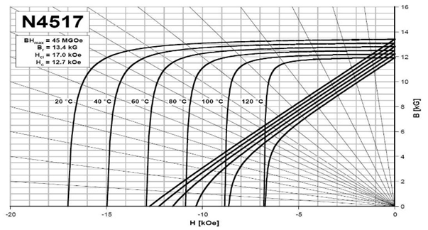
Figure 1 N4517 intrinsic and normal BH curves at different temperatures.
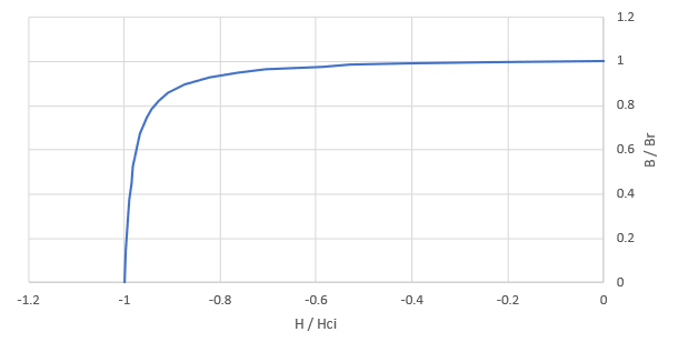
Figure 2 All normalized intrinsic BH curves for N4517 coincide each other.
Finally, the normal BH curve in the second and the third quadrants can be further derived through the conversion using equation (1).
Parameters T0, α1, and α2 for temperature dependent factor P(T) can be specified via Thermal Modifier of the Relative Permeability field, and parameters T0, β1, and β2 for temperature dependent factor Q(T) can be specified via Thermal Modifier of the Magnitude field, as shown in Figure 3.
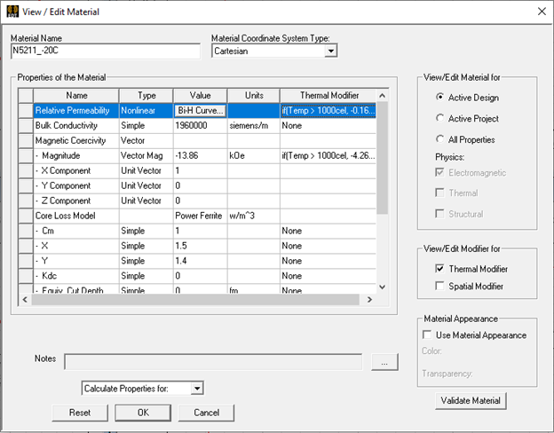
Figure 3: Thermal Modifiers for temperature dependent factors of Br via Relative Permeability field and Hci via Magnitude field, respectively.
Interpolating from Multiple Demagnetizing Curves
If the intrinsic BH curves are not shape-preserved, or temperature-dependent parameters are not available, two or more intrinsic BH curves at various reference temperatures are required. Suppose there are m inputs of temperature-dependent intrinsic demagnetization curves in the form of


where T0, Tk, and Tm (T0 < Tk < Tm) are reference temperatures at which demagnetization curves were measured. The flux density of the end point bkNk is the residual br_k for curve k.
The number of (hki, bki) points, Nk +1, in each demagnetization curve can be different.
In Maxwell, if the local temperature of temperature-dependent nonlinear magnetic material is T, the local demagnetization curve can be obtained by interpolation:
If T ≤ T0, the demagnetization curve at temperature T0 is returned as the interpolated demagnetization curve.
If T ≥Tm, the demagnetization curve at temperature Tm is returned as the interpolated demagnetization curve.
If Tk < T ≤ Tk+1, the interpolated demagnetization curve at temperature T can be derived by following steps:
- Get temperature interpolating coefficient: cT = (T − Tk) / (Tk+1 − Tk).
- Get interpolated intrinsic coercivity: hci = (1 − cT) hci_k + cT hci_k+1.
- Get interpolated residual: br = (1 − cT) br_k + cT br_k+1.
- Derive demagnetization curve at temperature T using the shape preserving algorithm based on the curve at Tk, which is expressed as (hki•Q0, bki•P0), where Q0 = hci / hci_k, and P0 = br / br_k.
- Derive demagnetization curve at temperature T using the shape preserving algorithm based on the curve at Tk+1. which is expressed as (hk+1i•Q1, bk+1i•P1), where Q1 = hci / hci_k+1, and P1 = br / br_k+1.
- Derive the weighted average curve from the curve expressed by (hki•Q0, bki•P0) and the curve expressed by (hk+1 i•Q1, bk+1 i•P1) with weighting factors of (1 − cT) and cT, respectively.
We can input temperature-dependent demagnetization curves in both normal and intrinsic formats. When normal demagnetization curves are input, we will transfer them to intrinsic curves and extend them with additional estimated data sets. Since the extended curve parts are approximated, it is suggested to directly input intrinsic curves with different temperatures as basic curves for interpolation, if they are available.
For example, the material Ferrite Y30 has BH curves with Br decreasing and Hci increasing as temperature increasing, as shown in Figure 4. If we input two intrinsic curves of the minimum and maximum temperatures, we can interpolate the intrinsic curves of other temperatures, and derive normal curves, as shown in Figure 5.
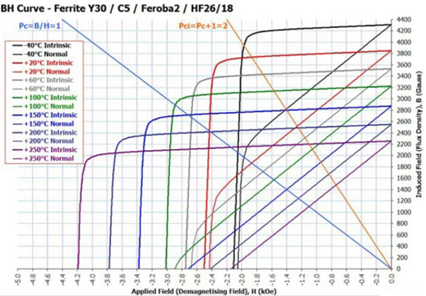
Figure 4: Temperature-dependent BH curves of Ferrite Y30

Figure 5: Input two intrinsic curves in solid lines, interpolated intrinsic curves in short-dashed lines, and derived normal curves in long-dashed lines.
If intrinsic curves are not available, we need to input three normal curves with minimum and maximum temperatures, as well as the curve with maximum Hc. In such cases, the estimated and interpolated intrinsic curves, and derive normal curves, are shown in Figure 6.
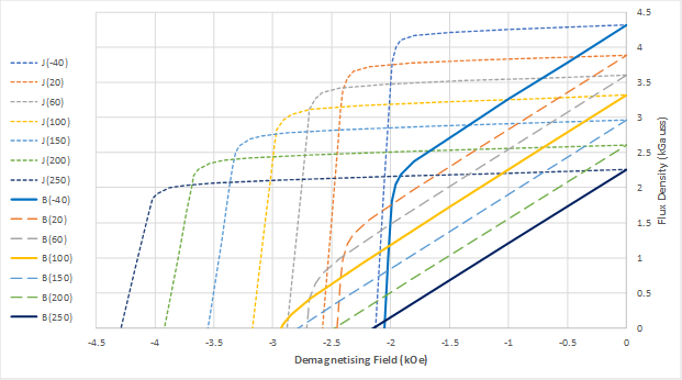
Figure 6: Input three normal curves in solid lines, estimated and interpolated intrinsic curves in short-dashed lines, and derived normal curves in long-dashed lines.
Multiple temperature-dependent normal or intrinsic demagnetization curves can be specified via BH Curve editing panel, as shown in Figure 7. In the drop-down menu menu of the Temperature field, select Edit Temperature Dependency to launch Edit Temperature Dependency dialog box, in which all temperature references for all magnetization curves can be specified. Then, each demagnetization curve related to each reference temperature can be input in the BH Curve panel.
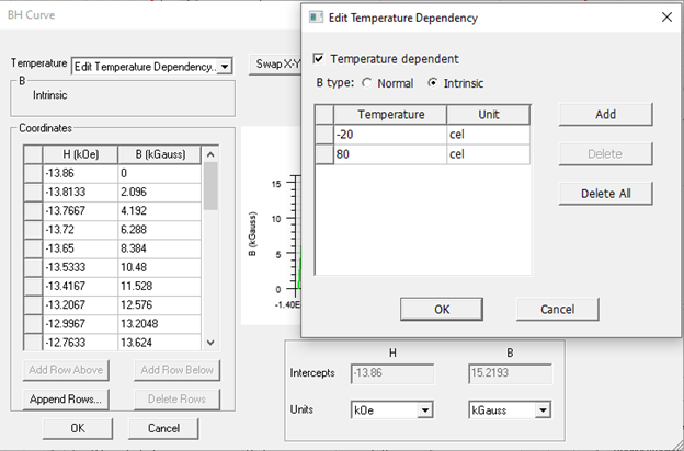
Figure 7: BH Curve panel to specify multiple temperature-dependent demagnetization curves