Magnetostatic Theory

The magnetostatic field simulator solves for the magnetic vector potential, A_z(x,y) in this field equation:

where

A_z(x,y) is the z component of the magnetic vector potential.
J_z(x,y) is the DC current density field flowing in the direction of transmission.
m_r is the relative permeability of each material.
m₀ is the permeability of free space.

Given J_z(x,y) as an excitation, the magnetostatic field simulator computes the magnetic vector potential at all points in space.

Note: In general, both J and A are vectors. However, J is assumed to only have a z-component. A consequence of this is that A only has a z-component as well. Both quantities can therefore be treated as scalars.

The equation that the magnetostatic field solver computes is derived from Ampere’s law, which is

Ñ x H = J

and from Maxwell’s equation, Ñ• B = 0.

Because H = B/m_rm₀, then

Because B = Ñ x A, due to Ñ• B = 0, then

The magnetostatic field simulator solves this equation using the finite element method.

After A_z(x,y) is computed, the magnetic flux density, B, and the magnetic field, H, can then be computed using the relationships B = Ñ x A, and H for linear materials is H = B/m_rm₀.

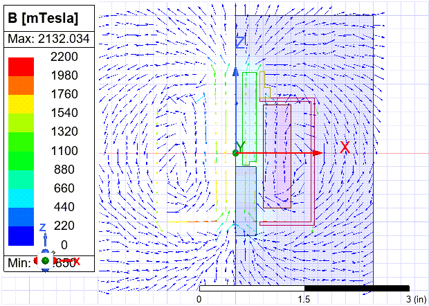
Both B and H lie in the xy cross-section being analyzed. An arrow plot of a B-field generated by the magnetostatic field simulator is shown below: