Large Scale DSO Theory

The parametric analysis command in Desktop computes simulation results as a function of model parameters, such as geometry dimensions, material properties and excitations. The parametric analysis is either performed on a local machine, where each variation is analyzed serially by a single engine, or distributed across machines through a DSO license. Desktop's DSO analysis runs multiple engines in parallel, thus generating results in a shorter time. In the Regular DSO algorithm, the parametric analysis job (Desktop) runs on master node, which in turn launches one or more distributed-parallel engines on each machine allocated to the job. Desktop distributes parametric variations among these engines running in parallel. As variations are solved, the progress/messages and variation results are sent back to Desktop, where they are persisted into the common results database on master node, as illustrated below:

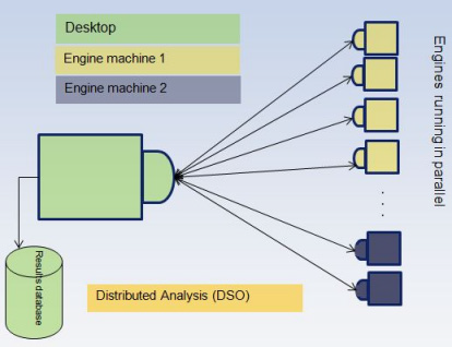
A single engine can now span multiple machines with auto multi-level DSO.

Regular DSO Bottleneck

As per above illustration, Regular DSO's speedup is limited by the resources of the centralized 'Desktop' bottleneck. It's been observed that DSO becomes unreliable at a certain point, as the number of engines and number of variations is increased. The term ‘large scale parallel’ can be used to define this tipping point. For a given model, a ‘large-scale parallel’ job denotes scenarios, in terms of the number of distributed-parallel engines and the number of parametric variations, where the Regular DSO runs into centralized bottlenecks that result in one or both of: progressively smaller speedups, unreliability.

With the advent of economical availability and timely provisioning of compute resources, product designers have access to large compute clusters to run their simulations. And they are throwing larger and larger number of compute resources at simulation jobs, in order to obtain results faster. The parametric DSO needs to meet this challenge and target linear speedup for 'large-scale parallel' jobs. The Large Scale DSO feature is targeted toward 100% reliability and linear speedup of large-scale parallel DSO jobs.

Key Algorithms/Concepts for Large Scale DSO

• Embarrassingly Parallel algorithm: Large Scale DSO exploits the embarrassingly parallel nature of parametric runs. The solve of each variation is made fully independent of another variation, by replacing Regular DSO's centralized database with per-engine distributed databases

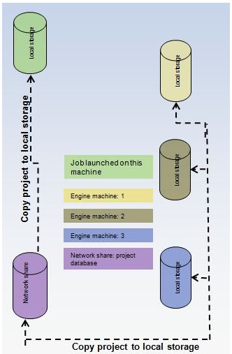
• Distributed databases: For each distributed-parallel engine, the database of the input model is cloned to local storage of engine's compute node (as illustrated in the following picture). Parallel analysis is performed on these cloned models and the analysis results also go the corresponding location on local storage. As each engine has its own database, there is no ‘shared database’ contention between any two engines. There is negligible network traffic as analysis/computations are contained in a single machine and use just the ‘local resources’.

• Hierarchical activation of engines: In the Large Scale DSO algorithm, engine activation is done hierarchically, where the overhead of launching of engines is also shared across the nodes. Such hierarchical activation improves reliability of the activation phase of large-scale parallel jobs. A new 'desktopjob' program encapsulates hierarchical activation, as illustrated in the following pictures. In this approach, the 'root' desktopjob (Root DJ) activates a 'level-one' child desktopjob (DJ(L1)) for each unique node allocated to the DSO job. Each level-one desktopjob activates one or more 'leaf' desktopjobs (DJ(L2)) equal to the number of distributed engines per node. A leaf desktopjob in turn runs Desktop in batch mode, to perform local-machine parametric analysis to solve the variations assigned to this engine.
• Decentralized Load balancing: A parametric table is divided into regions of equal number of variations, with the number of regions equal to the number of engines. In the following illustration, the analysis of 30 parametric variations is distributed among 5 engines. Each engine solves it's assigned region as a ‘local machine’ parametric analysis. Large Scale DSO job is considered done once all engines are done with their assigned variations.
• Distributed results postprocessing: As engine is done with the solve of a variation, it extracts results for the solved variation before progressing to the analysis of next variation. The extracted results are saved to the local storage. When the engine is done with analysis of all variations, the extracted results are transferred from local storage to the results folder of the input project.

Redistribution Feature

• Large Scale Distributed Solve Operation could submit a parametric setup to be solved in multiple machines, each machine may launch multiple EM-Desktop processes to solve the assigned variations(Design Points). ​ Variations are distributed to each task(EM-Desktop process) equally, regardless of the machine hardware and each variation’s complexity. That may result in some tasks finishing earlier than others, in some extreme case some tasks may hours behind fastest task.​

• Now, redistribution occurs when a task finished its own assignment, it calls back to the L2 to ask for new assignment, L2 forward the request to L1, L1 forward it to L0, L0 may pick one of the slow task to remove some variations or return with no more assignment. ​When a task is picked to remove unsolved variation, L0 calls L1(may be different L1), L1 forward it to the selected L2, L2 makes a request to the EM-Desktop to remove some variations from its queue. EM-Desktop returns the removed variation indexes, or error code if it fails.​ In L0 if error is returned, it marks the selected task failed to respond the remove request, to void picking it again.​ L0 returns the result through L1-L2 back the EM-Desktop.​

• The Ansys Electronics Desktop will ​enqueue the new assignment and then start solving those new variations.​ If the return data indicates error, it makes another call to L2 to get a new assignment.​ If no more variations return, the Ansys Electronics Desktop finishes the simulation and exits.