
Creating Rectangular Contour Plots
This is an x-y-z graph of results. Any data that you can current plot in 3D is a candidate for a contour plot.
- Select Maxwell > Results > Create <type> Report, (or right-click on Results on the Project tree and select Create <type> Report), and select Rectangular Contour plot from the report type menu.
- In the Context section make selections from the following field or fields, depending on the design and solution type.
-
Solution field with a drop down selection list. This lists the available setups and sweeps. As a minimum, the LastAdaptive solution and AdaptivePass solution is available to choose.
The AdaptivePass solution context can be selected to allow any value or parameter to be plotted versus the adaptive pass. This function is usually used to evaluate the convergence of the solution.
- Parameter field with a drop down selection list. Whether this field appears, and the parameters listed depend on the Solution type and the <type> selected.
-
For Eddy Current projects only: Matrix field with a drop-down selection list containing options for plotting matrix and reduce matrix parameters.
Note: In Maxwell Eddy Current designs, the user can create matrix parameters, which will cause the solver to produce an impedance matrix for the selected excitations. In addition, the user can group (wire) two or more excitations to one excitation in either a series or parallel connection referred to as a reduce matrix. The Matrix field appears only if a matrix entry is selected in the Parameter field. (Refer to Assigning a Matrix for information on creating a matrix and Assigning a Reduce Matrix for information on creating reduced matrix parameters for Eddy Current designs.)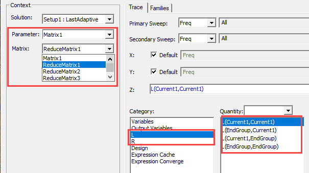
- For Fields and Noise Vibration reports: Geometry field with a drop down selection list. This applies the quantity to a specific geometry.
- Under the Trace tab Z Component area, specify the information to plot as contours:
- In the Category list, click the type of information to plot.
- In the Quantity list, click the value to plot.
- In the Function list, click the mathematical function of the quantity to plot.
- The Value field displays the currently specified Quantity and Function. You can edit this field directly.
- The Range Function button opens the Set Range Function dialog box, which applies currently specified Quantity and Function.
- On the Trace tab Y (Secondary sweep) lines, specify the information to plot along the y axis in one of the following ways:
- Select the sweep variable to use from the Secondary Sweep drop down list.
- If sweeps are available, you can select the browse button to display a dialog that lets you select particular values. The quantity will be plotted against the primary sweep variable listed.
- On the Trace tab X (Primary sweep) lines, specify the information to plot along the x-axis in one of the following ways:
- Select the sweep variable to use from the Primary Sweep drop down list.
- If sweeps are available, you can also select the browse [...] button to display a dialog box that lets you select particular sweep values, specify a range of sweep values (for Time sweeps), or Use all values (the default setting). The quantity will be plotted against the primary sweep variable listed.
- On the Families tab, confirm or modify the sweep variables that will be plotted.
- Click New Report.
- Optionally, add another trace to the plot by following the procedure above, using Add Trace rather than New Report.
The Report dialog appears.
This creates a new report in Project Manager tree, displays the report with the defined trace, and enables the Add Trace button on the Report dialog box. The default name is based on the Report Category you selected, for example, Force Plot n or Output Variables Plot n). You can edit the plot names in the project tree and the plot header text in the report synchronizes.
The function of the selected quantity or quantities will be plotted against the values you specified on an x-y-z graph. The plot is listed under Results in the Project Manager tree. When you select the traces or plots, their properties are displayed in the Properties window. These properties can be edited directly to modify the plot.