Turbulence
Eight turbulence models are available in Ansys Icepak: the zero-equation (mixing-length) model, the two-equation (standard  ) model, the RNG
  model, the realizable
  model, the enhanced two-equation (standard
  with enhanced wall treatment) model, the enhanced RNG
  model, the enhanced realizable
  model, the Spalart-Allmaras model and the
  SST model.
Zero-Equation Turbulence Model
The mixing-length zero-equation turbulence model (also known as the algebraic model) uses the following relation to calculate turbulent viscosity,  :
:
Equation 7

The mixing length,  , is defined as
Equation 8

where  is the distance from the wall and the von Kármán constant
  = 0.419.
 is the modulus of the mean rate-of-strain tensor, defined as
Equation 9

with the mean strain rate  given by
Equation 10

Advanced Turbulence Models
In turbulence models that employ the Boussinesq approach, the central issue is how the eddy viscosity is computed. The model proposed by Spalart and Allmaras [26] solves a transport equation for a quantity that is a modified form of the turbulent kinematic viscosity.
The standard  , RNG and realizable
  models have similar forms, with transport equations for
  and
and  . The major differences in the models are as follows:
-
the method of calculating turbulent viscosity
- the turbulent Prandtl numbers governing the turbulent diffusion of
 and
and 
-
the generation and destruction terms in the
 equation
This section describes the Reynolds-averaging method for calculating turbulent effects and provides an overview of the issues related to choosing an advanced turbulence model in Icepak. The transport equations, methods of calculating turbulent viscosity, and model constants are presented separately for each model. The features that are essentially common to both models follow, including turbulent production, generation due to buoyancy, and modeling heat transfer.
Reynolds (Ensemble) Averaging
The advanced turbulence models in Ansys Icepak are based on Reynolds averages of the governing equations. In Reynolds averaging, the solution variables in the instantaneous (exact) Navier-Stokes equations are decomposed into the mean (ensemble-averaged or time-averaged) and fluctuating components. For the velocity components:
Equation 11

where  and
and  are the mean and instantaneous velocity components (
 = 1, 2, 3).
Likewise, for pressure and other scalar quantities:
Equation 12

where  denotes a scalar such as pressure or energy. Substituting expressions of this form for the flow variables into the instantaneous continuity and momentum equations and taking a time (or ensemble) average (and dropping the overbar on the mean velocity,
  ) yields the ensemble-averaged momentum equations. They can be written in Cartesian tensor form as:
Equation 13

Equation 14

Equation 15

These “Reynolds stresses”,
 , must be modeled in order to close Equation 15,
 For variable-density flows, Equation 13 and Equation 15 can be interpreted as Favre-averaged Navier-Stokes equations [8], with the velocities representing mass-averaged values. As such, Equation 13 and Equation 15 can be applied to density-varying flows.
Boussinesq Approach
The Reynolds-averaged approach to turbulence modeling requires that the Reynolds stresses in Equation 15 be appropriately modeled. A common method employs the Boussinesq hypothesis [8] to relate the Reynolds stresses to the mean velocity gradients:
Equation 16

The Boussinesq hypothesis is used in the Spalart-Allmaras model and the  models. The advantage of this approach is the relatively low computational cost associated with the computation of the turbulent viscosity,
  . In the case of the Spalart-Allmaras model, only one additional transport equation (representing turbulent viscosity) is solved. In the case of the
  models, two additional transport equations (for the turbulence kinetic energy,
  , and the turbulence dissipation rate,
  ) are solved, and
  is computed as a function of
  and
and  . The disadvantage of the Boussinesq hypothesis as presented is that it assumes
  is an isotropic scalar quantity, which is not strictly true.
Choosing an Advanced Turbulence Model
This section provides an overview of the issues related to the advanced turbulence models provided in Icepak.
The Spalart-Allmaras Model
The Spalart-Allmaras model is a relatively simple one-equation model that solves a modeled transport equation for the kinematic eddy (turbulent) viscosity. This embodies a relatively new class of one equation models in which it is not necessary to calculate a length scale related to the local shear layer thickness. The Spalart-Allmaras model was designed specifically for aerospace applications involving wall-bounded flows and has been shown to give good results for boundary layers subjected to adverse pressure gradients. It is also gaining popularity for turbomachinery applications.
On a cautionary note, however, the Spalart-Allmaras model is still relatively new, and no claim is made regarding its suitability to all types of complex engineering flows. For instance, it cannot be relied on to predict the decay of homogeneous, isotropic turbulence. Furthermore, one-equation models are often criticized for their inability to rapidly accommodate changes in length scale, such as might be necessary when the flow changes abruptly from a wall-bounded to a free shear flow.
The Standard  Model
Model
The simplest “complete models” of turbulence are two-equation models in which the solution of two separate transport equations allows the turbulent velocity and length scales to be independently determined. The standard  model in Icepak falls within this class of turbulence model and has become the workhorse of practical engineering flow calculations in the time since it was proposed by Launder and Spalding [18]. Robustness, economy, and reasonable accuracy for a wide range of turbulent flows explain its popularity in industrial flow and heat transfer simulations. It is a semiempirical model, and the derivation of the model equations relies on phenomenological considerations and empiricism.
As the strengths and weaknesses of the standard  model have become known, improvements have been made to the model to improve its performance. One of these variants is available in Icepak: the RNG k-ε model [ 29 ].
The RNG  Model
Model
The RNG  model was derived using a rigorous statistical technique (called renormalization group theory). It is similar in form to the standard
  model, but includes the following refinements:
-
The RNG model has an additional term in its ε equation that significantly improves the accuracy for rapidly strained flows.
-
The effect of swirl on turbulence is included in the RNG model, enhancing accuracy for swirling flows.
-
The RNG theory provides an analytical formula for turbulent Prandtl numbers, while the standard
 model uses user-specified, constant values.
 -
While the standard
 model is a high-Reynolds-number model, the RNG theory provides an analytically-derived differential formula for effective viscosity that accounts for low-Reynolds number effects.
These features make the RNG  model more accurate and reliable for a wider class of flows than the standard
  model.
The Realizable  Model
Model
The realizable  model is a relatively recent development and differs from the standard
  model in two important ways:
-
The realizable
 model contains a new formulation for the turbulent viscosity.
 -
A new transport equation for the dissipation rate,
 , has been derived from an exact equation for the transport of the mean-square vorticity fluctuation.
The term “realizable” means that the model satisfies certain mathematical constraints on the Reynolds stresses, consistent with the physics of turbulent flows. Neither the standard k-ε model nor the RNG  model is realizable.
The Enhanced Two-Equation Models
The  models are primarily valid for turbulent core flows (that is, the flow in the regions somewhat far from walls). Consideration therefore needs to be given as to how to make these models suitable for wall-bounded flows.
Turbulent flows are significantly affected by the presence of walls. Obviously, the mean velocity field is affected through the no-slip condition that has to be satisfied at the wall. However, the turbulence is also changed by the presence of the wall in non-trivial ways. Very close to the wall, viscous damping reduces the tangential velocity fluctuations, while kinematic blocking reduces the normal fluctuations. Toward the outer part of the near-wall region, however, the turbulence is rapidly augmented by the production of turbulence kinetic energy due to the large gradients in mean velocity.
The near-wall modeling significantly impacts the fidelity of numerical solutions, inasmuch as walls are the main source of mean vorticity and turbulence. It is in the near-wall region where the solution variables have large gradients and where the momentum and other scalar transports are the greatest. Therefore, accurate representation of the flow in the near-wall region determines successful predictions of wall-bounded turbulent flows.
Numerous experiments have shown that the near-wall region can be largely subdivided into three layers. In the innermost layer, called the viscous sublayer, the flow is almost laminar, and the (molecular) viscosity plays a dominant role in momentum and heat or mass transfer. In the outer layer, called the fully-turbulent layer, turbulence plays a major role. Finally, there is an interim region between the viscous sublayer and the fully turbulent layer where the effects of molecular viscosity and turbulence are equally important.
To more accurately resolve the flow near the wall, the enhanced two-equation models combine three  models (standard, RNG and realizable) with enhanced wall treatment.
Enhanced Wall Treatment
Enhanced wall treatment is a near-wall modeling method that combines a two-layer model with enhanced wall functions [ 3 9 14 15 27 28 ].
In the two-layer model, the viscosity-affected near-wall region is completely resolved all the way to the viscous sublayer. The two-layer approach is an integral part of the enhanced wall treatment and is used to specify both  and the turbulent viscosity in the near-wall cells. In this approach, the whole domain is subdivided into a viscosity-affected region and a fully-turbulent region. The demarcation of the two regions is determined by a wall-distance-based, turbulent Reynolds number.
If the near-wall mesh is fine enough to be able to resolve the laminar sublayer (typically  ), then the enhanced wall treatment will be identical to the traditional two-layer zonal model. However, the restriction that the near-wall mesh must be sufficiently fine everywhere might impose too large a computational requirement. Ideally, then, one would like to have a near-wall formulation that can be used with coarse meshes (usually referred to as wall-function meshes) as well as fine meshes (low-Reynolds-number meshes). In addition, excessive error should not be incurred for intermediate meshes that are too fine for the near-wall cell centroid to lie in the fully turbulent region, but also too coarse to properly resolve the sublayer.
To achieve the goal of having a near-wall modeling approach that will possess the accuracy of the standard two-layer approach for fine near-wall meshes and will not significantly reduce accuracy for wall-function meshes, Icepak combines the two-layer model with enhanced wall functions to result in the enhanced wall treatment.
Computational Effort: CPU Time and Solution Behavior
The standard  model clearly requires more computational effort than the Spalart-Allmaras model since an additional transport equation is solved. The realizable
  model requires only slightly more computational effort than the standard
  model. However, due to the extra terms and functions in the governing equations and a greater degree of nonlinearity, computations with the RNG
  model tend to take 10-15% more CPU time than with the standard
  model.
Aside from the time per iteration, the choice of turbulence model can affect the ability of Ansys Icepak to obtain a converged solution. For example, the standard  model is known to be slightly over-diffusive in certain situations, while the RNG
  model is designed such that the turbulent viscosity is reduced in response to high rates of strain. Because diffusion has a stabilizing effect on the numerics, the RNG model is more likely to be susceptible to instability in steady-state solutions. However, this should not necessarily be seen as a disadvantage of the RNG model, since these characteristics make it more responsive to important physical instabilities such as time-dependent turbulent vortex shedding.
The Spalart-Allmaras Model
In its original form, the Spalart-Allmaras model is effectively a low-Reynolds-number model, requiring the viscous-affected region of the boundary layer to be properly resolved. In Icepak, however, the Spalart-Allmaras model has been implemented to use wall functions when the mesh resolution is not sufficiently fine. This might make it the best choice for relatively crude simulations on coarse meshes where accurate turbulent flow computations are not critical. Furthermore, the near-wall gradients of the transported variable in the model are much smaller than the gradients of the transported variables in the  models. This might make the model less sensitive to numerical error when non-layered meshes are used near walls.
Transport Equation for the Spalart-Allmaras Model
The transported variable in the Spalart-Allmaras model,  , is identical to the turbulent kinematic viscosity except in the near-wall (viscous-affected) region. The transport equation for
  is
is
Equation 17

where  is the production of turbulent viscosity and
  is the destruction of turbulent viscosity that occurs in the near-wall region due to wall blocking and viscous damping.
  ̃ and
̃ and  are constants and
  is the molecular kinematic viscosity.
  is a user-defined source term. Note that since the turbulence kinetic energy
  is not calculated in the Spalart-Allmaras model, the last term in Equation 16 is ignored when estimating the Reynolds stresses.
Modeling the Turbulent Viscosity
The turbulent viscosity,  , is computed from
Equation 18

where the viscous damping function,  , is given by
Equation 19

and
Equation 20

Modeling the Turbulent Production
The production term,  , is modeled as
Equation 21

where
Equation 22

and
Equation 23

 and
and  are constants,
  is the distance from the wall, and
  is a scalar measure of the deformation tensor. By default in Icepak, as in the original model proposed by Spalart and Allmaras,
  is based on the magnitude of the vorticity:
Equation 24

where  is the mean rate-of-rotation tensor and is defined by
Equation 25

The justification for the default expression for  is that, for the wall-bounded flows that were of most interest when the model was formulated, turbulence is found only where vorticity is generated near walls. However, it has since been acknowledged that one should also take into account the effect of mean strain on the turbulence production, and a modification to the model has been proposed [6] and incorporated into Icepak.
This modification combines measures of both rotation and strain tensors in the definition of  :
:
Equation 26

where
Equation 27

with the mean strain rate,  , defined as
Equation 28

Including both the rotation and strain tensors reduces the production of eddy viscosity and consequently reduces the eddy viscosity itself in regions where the measure of vorticity exceeds that of strain rate. One such example can be found in vortical flows, that is, flow near the core of a vortex subjected to a pure rotation where turbulence is known to be suppressed. Including both the rotation and strain tensors more correctly accounts for the effects of rotation on turbulence. The default option (including the rotation tensor only) tends to overpredict the production of eddy viscosity and hence overpredicts the eddy viscosity itself in certain circumstances.
Modeling the Turbulent Destruction
The destruction term is modeled as
Equation 29

where
Equation 30

Equation 31

Equation 32

 ,
,  , and
, and  are constants, and
  is given by Equation 22. Note that the modification described above to include the effects of mean strain on
  will also affect the value of
  used to compute
  .
.
Model Constants
The model constants  and
and  have the following default values [26]:
Equation 33

Equation 34

Wall Boundary Conditions
At walls, the modified turbulent kinematic viscosity,  , is set to zero.
When the mesh is fine enough to resolve the laminar sublayer, the wall shear stress is obtained from the laminar stress-strain relationship:
Equation 35

If the mesh is too coarse to resolve the laminar sublayer, it is assumed that the centroid of the wall-adjacent cell falls within the logarithmic region of the boundary layer, and the law-of-the-wall is employed:
Equation 36

where  is the velocity parallel to the wall,
  is the shear velocity,
  is the distance from the wall,
  is the von Kármán constant (0.4187), and
  = 9.793.
Convective Heat and Mass Transfer Modeling
In Icepak, turbulent heat transport is modeled using the concept of Reynolds’ analogy to turbulent momentum transfer. The modeled energy equation is thus given by the following:
Equation 37

where  , in this case, is the thermal conductivity,
  is the total energy, and
  is the deviatoric stress tensor, defined as
Equation 38

The term involving  represents the viscous heating. The default value of the turbulent Prandtl number is 0.85. Turbulent mass transfer is treated similarly, with a default turbulent Schmidt number of 0.7.
Wall boundary conditions for scalar transport are handled analogously to momentum, using the appropriate law-of-the-wall.
Two-Equation (Standard  ) Turbulence Model
The two-equation turbulence model (also known as the standard  model) is more complex than the zero-equation model. The standard
  model is a semi-empirical model based on model transport equations for the turbulent kinetic energy (
 ) and its dissipation rate (
 ). The model transport equation for
  is derived from the exact equation, while the model transport equation for
  is obtained using physical reasoning and bears little resemblance to its mathematically exact counterpart.
In the derivation of the standard  model, it is assumed that the flow is fully turbulent, and the effects of molecular viscosity are negligible. The standard
  model is therefore valid only for fully turbulent flows.
Transport Equations for the Standard  Model
Model
The turbulent kinetic energy, , and its rate of dissipation,
  , are obtained from the following transport equations:
Equation 39

and
Equation 40

In these equations,  represents the generation of turbulent kinetic energy due to the mean velocity gradients, calculated as described later in this section.
  is the generation of turbulent kinetic energy due to buoyancy, calculated as described later in this section.
  ,
, , and
, and  are constants.
  and
and  are the turbulent Prandtl numbers for
  and
and  , respectively.
Modeling the Turbulent Viscosity
The eddy or turbulent viscosity turbulent viscosity,  , is computed by combining
  and
and  as follows:
Equation 41

where  is a constant.
Model Constants
The model constants  ,
,  .
.  ,
,  , and
, and  have the following default values [18] :
Equation 42

These default values have been determined from experiments with air and water for fundamental turbulent shear flows including homogeneous shear flows and decaying isotropic grid turbulence. They have been found to work fairly well for a wide range of wall-bounded and free shear flows.
The RNG  Model
Model
The RNG-based  turbulence model is derived from the instantaneous Navier-Stokes equations, using a mathematical technique called renormalization group (RNG) methods. The analytical derivation results in a model with constants different from those in the standard
  model, and additional terms and functions in the transport equations for
  and
and  . A more comprehensive description of RNG theory and its application to turbulence can be found in .renormalization group (RNG) theory [4].
Transport Equations for the RNG ε Model
The RNG  model has a similar form to the standard
  model:
Equation 43

and
Equation 44

In these equations,  represents the generation of turbulent kinetic energy due to the mean velocity gradients, calculated as described later in this section.
  is the generation of turbulent kinetic energy due to buoyancy, calculated as described later in this section. The quantities
  and
and  are the inverse effective Prandtl numbers for
  and
and  , respectively.
Modeling the Effective Viscosity
The scale elimination procedure in RNG theory results in a differential equation for turbulent viscosity:
Equation 45

where
Equation 46

Equation 45 is integrated to obtain an accurate description of how the effective turbulent transport varies with the effective Reynolds number (or eddy scale), allowing the model to better handle low-Reynolds-number low-Reynolds-number flows and near-wall flows.
In the high-Reynolds-number limit, Equation 45 gives
Equation 47

with  = 0.0845, derived using RNG theory. It is interesting to note that this value of
  is very close to the empirically-determined value of 0.09 used in the standard
  model.
In Icepak, the effective viscosity is computed using the high-Reynolds-number form in Equation 47.
Calculating the Inverse Effective Prandtl Numbers
The inverse effective Prandtl numbers  and
and  are computed using the following formula derived analytically by the RNG theory:
Equation 48

where  = 1.0. In the high-Reynolds-number limit (
 #1),
#1),  =
=  ≈ 1.393.
The  Term in the
  Equation
The main difference between the RNG and standard  models lies in the additional term in the
  equation given by
Equation 49

where  ,
,  = 4.38,
  = 0.012.
The effects of this term in the RNG  equation can be seen more clearly by rearranging Equation 44. Using Equation 49, the last two terms in Equation 44 can be merged, and the resulting
  equation can be rewritten as
Equation 50

where  is given by
Equation 51

In regions where  <<
<< , the
, the  term makes a positive contribution, and
  becomes larger than
  . In the logarithmic layer, for instance, it can be shown that
  ≈3.0, giving
  ≈ 2.0, which is close in magnitude to the value of
  in the standard
  model (1.92). As a result, for weakly to moderately strained flows, the RNG model tends to give results largely comparable to the standard
  model.
In regions of large strain rate (
 ), however, the R term makes a negative contribution, making the value of
  less than
  . In comparison with the standard
  model, the smaller destruction of
  augments
  , reducing
  and eventually the effective viscosity. As a result, in rapidly strained flows, the RNG model yields a lower turbulent viscosity than the standard
  model.
Thus, the RNG model is more responsive to the effects of rapid strain and streamline curvature than the standard  model, which explains the superior performance of the RNG model for certain classes of flows.
Model Constants
The model constants  and
and  in Equation 44 have values derived analytically by the RNG theory. These values, used by default in Icepak, are
  = 1.42,
  = 1.68.
Modeling Turbulent Production in the  Models
From the exact equation for the transport of  , the term
  , representing the production of turbulent kinetic energy, can be defined as
Equation 52

To evaluate  in a manner consistent with the Boussinesq hypothesis,
Equation 53

where  is the modulus of the mean rate-of-strain tensor, defined as
Equation 54

with the mean strain rate  given by
Equation 55

Effects of Buoyancy on Turbulence in the  Models
When a non-zero gravity field and temperature gradient are present simultaneously, the  models in Icepak account for the generation of
  due to buoyancy (
 in Equation 39 and Equation 43), and the corresponding contribution to the production of
  in Equation 40 and Equation 44.
The generation of turbulence due to buoyancy is given by
Equation 56

where  is the turbulent Prandtl number for energy. For the standard
  model, the default value of
  is 0.85. In the case of the RNG
  model,
  where
where  is given by Equation 48, but with
  . The coefficient of thermal expansion,
  , is defined as
Equation 57

It can be seen from the transport equation for  (Equation 39 or Equation 43) that turbulent kinetic energy tends to be augmented (
 0) in unstable stratification. For stable stratification, buoyancy tends to suppress the turbulence (
 <0). In Ansys Icepak, the effects of buoyancy on the generation of
  are always included when you have both a non-zero gravity field and a non-zero temperature (or density) gradient.
While the buoyancy effects on the generation of  are relatively well understood, the effect on
  is less clear. In Ansys Icepak, by default, the buoyancy effects on
  are neglected simply by setting Gb to zero in the transport equation for
  (Equation 40 or Equation 44).
The degree to which  is affected by the buoyancy is determined by the constant
  . In Icepak,
  is not specified, but is instead calculated according to the following relation [7]:
Equation 58

where  is the component of the flow velocity parallel to the gravitational vector and
  is the component of the flow velocity perpendicular to the gravitational vector. In this way,
  will become 1 for buoyant shear layers for which the main flow direction is aligned with the direction of gravity. For buoyant shear layers that are perpendicular to the gravitational vector,
  will become zero.
Convective Heat Transfer Modeling in the  Models
In Icepak, turbulent heat transport is modeled using the concept of Reynolds’ analogy to turbulent momentum transfer. The modeled energy equation is thus given by the following:
Equation 59

where  is the total energy and
  is the effective conductivity.
For the standard  model,
  is given by
Equation 60

with the default value of the turbulent Prandtl number set to 0.85.
For the RNG  model, the effective thermal conductivity is
Equation 61

where  is calculated from Equation 48, but with
  .
.
The fact that  varies with
  , as in Equation 48, is an advantage of the RNG
  model. It is consistent with experimental evidence indicating that the turbulent Prandtl number varies with the molecular Prandtl number and turbulence [17]. Equation 48 works well across a very broad range of molecular Prandtl numbers, from liquid metals (
 ) to paraffin oils (
 ), which allows heat transfer to be calculated in low-Reynolds-number regions. Equation 48 smoothly predicts the variation of effective Prandtl number from the molecular value (
 ) in the viscosity-dominated region to the fully turbulent value (
 = 1.393) in the fully turbulent regions of the flow.
 SST Model
The  SST model is based on the coupling of the SST
  transport equations, one for the intermittency and one for the transition onset criteria, in terms of momentum-thickness Reynolds number. An Ansys empirical correlation (Langtry and Menter) has been developed to cover standard bypass transition as well as flows in low-free-stream turbulence environments. The
  SST model can be used as a low Reynolds number turbulence model. It also exhibits good behavior in adverse pressure gradients and separating flow.
Transport Equations for the Transition SST Model
The transport equation for the intermittency  is defined as:
Equation 62

The transition sources are defined as follows:
Equation 63

where  is the strain rate magnitude,
  is an empirical correlation that controls the length of the transition region, and
  and
and  hold the values of 2 and 1, respectively. The destruction/relaminarization sources are defined as follows:
Equation 64

where  is the vorticity magnitude. The transition onset is controlled by the following functions:
Equation 65

Equation 66

Equation 67

 is the critical Reynolds number where the intermittency first starts to increase in the boundary layer. This occurs upstream of the transition Reynolds number
  ̃ and the difference between the two must be obtained from an empirical correlation. Both the
  and
and  correlations are functions of
  .
.
The constants for the intermittency equation are:
Equation 68

Separation-Induced Transition Correction
The modification for separation-induced transition is:
Equation 69

Here,  is a constant with a value of 2.
The model constants in Equation 69 have been adjusted from those of Menter et al. [XmenterICE] in order to improve the predictions of separated flow transition. The main difference is that the constant that controls the relation between  and
and  was changed from 2.193, its value for a Blasius boundary layer, to 3.235, the value at a separation point where the shape factor is 3.5 [XmenterICE]. The boundary condition for
  at a wall is zero normal flux, while for an inlet,
  is equal to 1.0.
The transport equation for the transition momentum thickness Reynolds number  ̃ is
̃ is
Equation 70

The source term is defined as follows:
Equation 71

Equation 72

Equation 73

Equation 74

The model constants for the  ̃ equation are:
Equation 75

The boundary condition for  ̃ at a wall is zero flux. The boundary condition for
  ̃ at an inlet should be calculated from the empirical correlation based on the inlet turbulence intensity.
The model contains three empirical correlations.  is the transition onset as observed in experiments. This has been modified from Menter et al.[XmenterICE] in order to improve the predictions for natural transition. It is used in Equation 70.
  is the length of the transition zone and is substituted in Equation 62.
  is the point where the model is activated in order to match both
  and
and  , and is used in Equation 66. At present, these empirical correlations are proprietary and are not given in this User’s guide.
Equation 76

The first empirical correlation is a function of the local turbulence intensity,  , and the Thwaites’ pressure gradient coefficient
  is defined as
Equation 77

where  is the acceleration in the streamwise direction.
Coupling the Transition Model and SST Transport Equations
The transition model interacts with the SST turbulence model by modification of the  -equation, as follows:
Equation 78

Equation 79

Equation 80

where  ̃ and
̃ and  are the original production and destruction terms for the SST model. Note that the production term in the ω -equation is not modified. The rationale behind the above model formulation is given in detail in Menter et al. [XmenterICE].
In order to capture the laminar and transitional boundary layers correctly, the mesh must have a  of approximately one. If the
  is too large (that is, > 5), then the transition onset location moves upstream with increasing
  . It is recommended that you use the bounded second order upwind based discretization for the mean flow, turbulence and transition equations.
Specifying Inlet Turbulence Levels
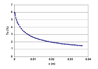
It has been observed that the turbulence intensity specified at an inlet can decay quite rapidly depending on the inlet viscosity ratio ( ) (and hence turbulence eddy frequency). As a result, the local turbulence intensity downstream of the inlet can be much smaller than the inlet value (see Figure 1: Exemplary Decay of Turbulence Intensity (Tu) as a Function of Streamwise Distance (x)). Typically, the larger the inlet viscosity ratio, the smaller the turbulent decay rate. However, if too large a viscosity ratio is specified (that is, > 100), the skin friction can deviate significantly from the laminar value. There is experimental evidence that suggests that this effect occurs physically; however, at this point it is not clear how accurately the transition model reproduces this behavior. For this reason, if possible, it is desirable to have a relatively low (that is,
  1 – 10) inlet viscosity ratio and to estimate the inlet value of turbulence intensity such that at the leading edge of the blade/airfoil, the turbulence intensity has decayed to the desired value. The decay of turbulent kinetic energy can be calculated with the following analytical solution:
Equation 81

For the SST turbulence model in the freestream the constants are:
Equation 82

The time scale can be determined as follows:
Equation 83

where  is the streamwise distance downstream of the inlet and
  is the mean convective velocity. The eddy viscosity is defined as:
Equation 84

The decay of turbulent kinetic energy equation can be rewritten in terms of inlet turbulence intensity ( ) and inlet eddy viscosity ratio (
 ) as follows:
Equation 85

Figure 1: Exemplary Decay of Turbulence Intensity (Tu) as a Function of Streamwise Distance (x)