Adaptive Mesh Refinement

Adaptive mesh refinement automatically generates accurate solutions. This meshing technique helps you focus on setting up your design efficiently rather than spending time in determining and creating the best mesh. To set up the design, you need only to create the geometry and specify material properties, boundary conditions, excitations, and the solution frequency.

This automatic adaptive mesh refinement technique differentiates HFSS from most electromagnetic simulators, which typically require extensive user controls to ensure that the generated mesh is suitable for simulation. Without the correct mesh, results from such simulators may be erroneous.

In HFSS, however, the automatically generated mesh accurately represents the electromagnetic characteristics of the design. HFSS determines the size and density of tetrahedra for optimal efficiency and accuracy. An initial mesh is generated and solved to produce error estimates of the solution. These error estimates are used to refine the mesh in high-error regions. Using this refined mesh, HFSS generates another solution and recomputes the error. This adaptive refinement process continues until HFSS converges to an accurate solution. Convergence is determined by monitoring a parameter from one adaptive pass to the next. The most common convergence criterion is to ensure that the difference in the S-parameter value between two consecutive solves is less than the specified magnitude. If you need to increase the accuracy, you can easily tighten the convergence criteria, and HFSS further refines the mesh.

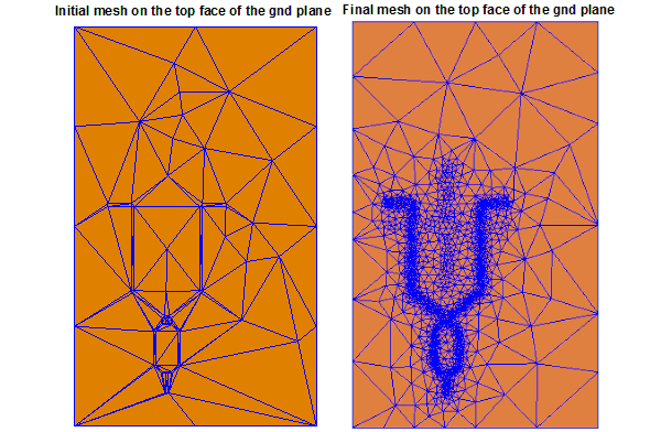
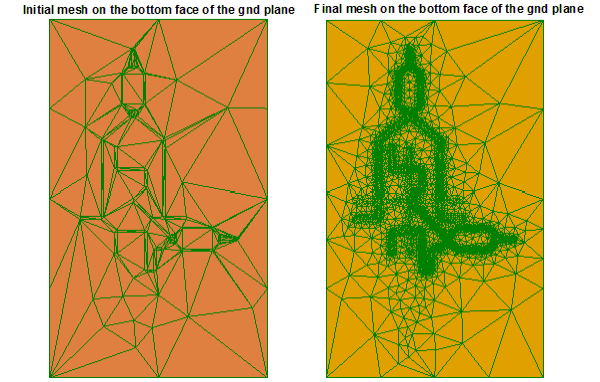
Adaptive refinement ensures that the mesh elements are sufficiently fine in those areas where strong electromagnetic fields exist and/or the field gradients are high. The mesh is coarser in the remaining areas. This process makes the mesh size appropriate and suitable for efficient simulations leading to highly accurate solutions.

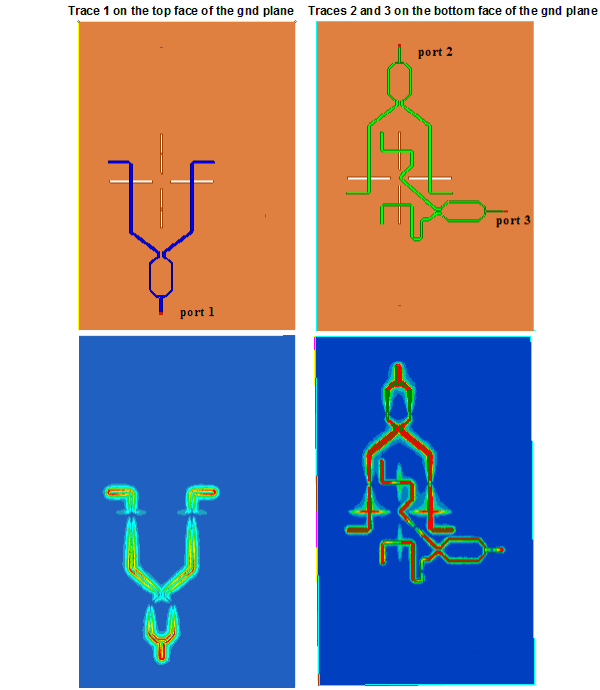
To illustrate, an aperture coupled microstrip filter design with three traces is shown below. One of the traces is located on one side of the ground plane, while the other two traces are located on the opposite side. The figures also show the resulting electric fields that develop for the design after the simulation is completed. The plots show the traces of the microstrip on both sides of the ground plane illuminated by the electromagnetic fields.

See both the initial and final meshes for these two layers and how they are automatically adapted by the adaptive refinement algorithm.