Transmit Jitter in QuickEye and VerifEye
Transmit jitter is variation in the location of edges. QuickEye and VerifEye can add the effects of transmit jitter, in combinations of Random (Gaussian), Uniform, Periodic, and Custom (user-defined) jitter.
QuickEye Jitter Calculation
QuickEye employs a Monte-Carlo method: each transition is displaced a random amount on the nominal time using a probability distribution that combines all specified Gaussian, Uniform, Periodic, and Custom jitter distributions. The Monte Carlo approach requires significant simulation time, since there is a different set of jittered transitions for each bit in the original stream.
VerifEye Jitter Calculation
The VerifEye method involves calculating the probability distribution function (PDF) for receiver voltage. VerifEye calculates a second probability distribution function that combines all specified Random (RJ), Uniform (UJ), Periodic (PJ), and Custom (user-defined, CJ) jitter distributions. The total jitter PDF (pTJ) is the convolution of the individual PDFs:

VerifEye translates the total jitter probability distribution function to the corresponding voltage PDF at each sample time. The voltage PDF has the same distribution as the jitter PDF. The mean of the voltage PDF is offset on the mean of the jitter distribution (always 0) by the value of the rising or falling step response. The width of the voltage PDF is the width of the jitter PDF scaled by the rate of change of the response at the sample time.

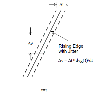
Figure 1. Transmit Jitter PDF Translated to Voltage PDF.
Figure 1 diagrams an arbitrary segment of a rising waveform, sampled at time t. The dotted lines indicate the maximum displacement of the waveform on the time axis due to transmit jitter, Dt. The exact shape of the jitter distribution is not shown. The corresponding spread in the voltage PDF due to jitter is shown as Dv. The slope of the rising wave at sample time t is:

The spread in the voltage PDF due to the spread in the jitter PDF is:

The next topics provide details on the PDFs for random (Gaussian), uniform, periodic, and custom (user-defined) transmit jitter.
Random Transmit Jitter
The Gaussian probability distribution function for variable x with mean m and standard deviation s is:

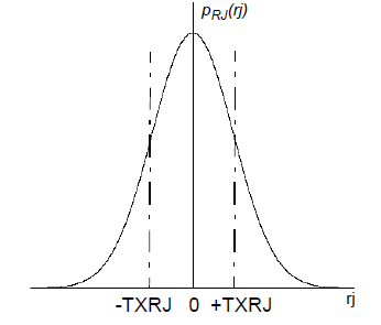
For QuickEye and VerifEye, the variable is the time value of the random jitter (t), the mean m is zero, and the standard deviation s is set to Eye Source entry TXRJ. The resulting PDF for random jitter is:

This PDF has the familiar normal curve, as shown in Figure 2:

Figure 2. Random Jitter PDF.
Uniform Transmit Jitter
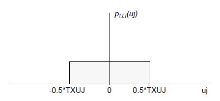
Uniform random jitter represents a distribution of offsets in time on the nominal edge location. The uniform distribution is centered on time uj=0 with bounds -0.5*TXUJ to +0.5*TXUJ, where TXUJ is the entry on the Eye Source (Figure 3).

Figure 3. Uniform Jitter PDF.
Uniform jitter is not common by itself, but can be used in combination with the other jitter distributions to more closely match measured values.
Periodic Transmit Jitter
Periodic jitter simulates the effect of variations in voltage such as those produced by sinusoidal noise. The periodic variation in voltage translates into a periodic variation in the location of the edges of the signals generated.
In the QuickEye and VerifEye implementation of periodic jitter, the frequency of the periodicity is ignored. The noise frequency is assumed to be uncorrelated to the clock frequency, and the phase of the periodic noise is basically a uniform random variable. The noise voltage is the sine of this variable, giving the following probability distribution (TXPJ is the Eye Source entry):

for |pj| < TXPJ, zero otherwise.
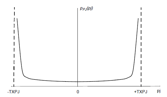
Figure 4 shows the shape of the periodic jitter PDF.
This probability distribution has peaks at
|pj| = TXPJ, and is
sometimes approximated as a bimodal or dual-Dirac distribution (but not
by QuickEye or VerifEye).

Figure 4. Periodic Jitter PDF
Custom or User-Defined Transmit Jitter
The user can specify a probability density function (PDF) for transmit jitter, to be combined with any other forms of jitter specified in the Eye source for both QuickEye and VerifEye. The PDF data is read on the file indicated by the TXCJ parameter on the Eye source.
The data in the jitter file are in two columns. The first column is the time in seconds. The time values may be positive or negative, and need not be centered around t=0. The Circuit solver automatically centers the mean value of the data at t=0 before doing the jitter calculation. The second column is the PDF value for each time. The PDF values must be greater than or equal to zero.
The Circuit solver automatically scales the PDF data such that the area underneath is unity, so no manual scaling is required.
The Circuit solver performs linear interpolation between the data points. Best results are obtained when the number of data points is large enough to minimize discontinuities of slope. The time axis should extend far enough to allow the PDF to drop to negligible values at both ends.
