Modeling Practice in HFSS

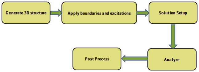
Typical modeling practice of creating and simulating a 3D model in HFSS involves the following steps:

Create model/geometry
Assign boundaries
Assign excitations
Assign solution setup
Validate and analyze
Perform post-processing operations

Every HFSS simulation involves, to some degree, all six of the above steps. It is not mandatory to follow these steps in the exact order, however, they constitute a good modeling practice.

The steps are described here.

1. Create Geometry

On the 3D Modeler, create the geometrical model that you want to analyze. The 3D modeler in HFSS has advanced features that enable you to parameterize a structure by creating variables and assigning values to them while defining geometric dimensions and material properties. A parameterized structure is very useful especially, when the final dimensions are not known or when the design needs to be modified for performance improvements.

You can also import 3D structures from mechanical drawing packages, such as SolidWorks®, Pro/E® or AutoCAD®. However, imported structures do not retain any history of how they were created so they will not be parameterizable upon import. You must manually modify an imported geometry, if you want to parameterize the structure.

2. Assign Boundaries

Assign boundary conditions in the next step. Boundaries are defined on 2D (sheet) objects specifically created for this purpose or on surfaces of 3D objects. Boundaries have a direct impact on the generated solutions. Depending upon the problem, HFSS offers different types of boundary conditions including Perfect E, Perfect H, Radiation, Primary, Secondary, Impedance, Finite Conductivity, PML, Layered Impedance, Anisotropic Impedance, and Lumped RLC.

Note: For more information about boundary conditions, see the chapter Assigning Boundaries in HFSS in the ANSYS Electronics Desktop help.

3. Assign Excitations

Excite the geometry by assigning excitations. Excitations are sources of electromagnetic fields in the design. HFSS has various options to generate incident fields that interact with a structure to produce the total fields. Some of these excitations are local sources residing within the structure such as wave ports and voltage sources while other excitations such as plane waves are created from local sources away from the structure. Excitations available in HFSS include wave port, lumped port, terminal, Floquet ports, incident wave, voltage source, current source, magnetic bias. There are several convenient rules that you can follow for proper creation and use of excitations to obtain highly accurate results in HFSS.

Note: For more information about excitations and the guidelines for defining them, see the chapter Assigning Excitations for HFSS in the Ansys Electronics Desktop help.

4. Assign Solution Setup

The next step is to create a solution setup. In this step, specify a solution frequency, the desired convergence criteria which include the maximum number of adaptive passes and the magnitude of maximum delta S. To generate a solution across a range of frequencies, define a frequency sweep.

5. Validate and Analyze

After performing the above four steps, the model can be validated and then analyzed if it passes the validation check. The time required for an analysis depends upon the model geometry, the solution frequency, and available computer resources. HFSS also comes with advanced High Performance Computing capability for accelerated performance and for solving large problems.

6. Post Processing

Perform post processing once the simulation runs to completion. Any field quantity or S,Y,Z parameter can be plotted in the post-processor. Additionally, if a parameterized model has been analyzed, families of curves can be created. For example, you can examine the S-parameters of the device modeled, far fields created by an antenna, or plot the electromagnetic fields in and around the structure.