
Advanced Complex Material Properties and Models
This chapter shows how HFSS can incorporate complex, anisotropic, and dispersive material properties. We provide examples showing two common dispersive models to represent high frequency metal behavior and superconductive material behavior well beneath the critical temperature. The two models are the Drude Model For Dispersive Metals for dispersive metals at very high frequencies and the Generalized Superconductive Model used to represent the electrical properties of superconductive materials well below the critical temperature. Both cases use frequency dependent project variables to provide the model.
Complex Material Properties
Complex material properties have been traditionally entered as either of the following: real relative permittivity, real relative permeability, electric/magnetic loss tangent, and conductivity. Though this is helpful for many industries, there are now many applications that benefit by having an entry of a real and an imaginary relative permittivity and permeability as well. In some applications, it is also helpful to have entry of a complex conductivity. HFSS now allows all of the above entries to aid in a high fidelity model of the material.
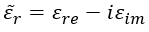
With a permittivity definition, the real part represents the phase velocity and propagation characteristics while the imaginary part represents the loss terms:
This expression can be expanded by adding the loss effects of metals via the conductivity:
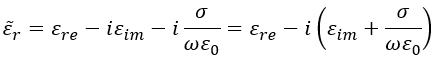
The above equation seems to be the most representative for complex relative permittivity. However, on occasion it can be useful to think in terms of complex conductivity rather than complex relative permittivity. An example is the Drude Model for dispersive metals at high frequencies.
Drude Model For Dispersive Metals
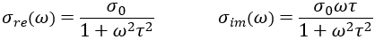
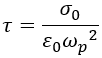
The Drude Model represents the high frequency electrical behavior of metals as a function of DC conductivity and the Plasma Frequency. This model is typically represented as a complex conductivity:
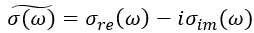
With a conductivity definition the real term represents the classic conductive loss while the imaginary part characterizes the phase velocity and propagation. This is a bit counter intuitive, but as the Helmholtz Equation accepts a single complex quantity to represent the phase velocity and loss, it follows that how we compartmentalize the terms simply aids in understanding.
 , and the mean collision time,

To enter these relations into HFSS you must create frequency dependent Project Variables. All Project Variables in HFSS are scoped such that they are visible to every design in the AEDT project and are prefixed with a “$” symbol. To create the project variables, go to Project > Project Variables... to see a list of existing project variables. Click Add on the project variable list for a dialog to enter names and values for each variable you need. The values here assume that the plasma frequency and mean collision time is known. When you have added the variables, the Project variable list will look like this:
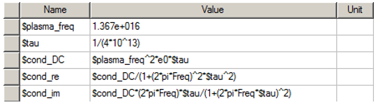
You can see above that the Project variables can be made a function of frequency using the built-in variable, Freq. This frequency variable automatically adapts the variable value based upon the frequency of solution.
To show the use of the complex conductivity entry, we will provide a comparison to published literature for a wide angle InfraRed Absorber FSS1. In the cited paper, the material properties of the FSS are given in terms of the plasma frequency, 1.367 * 1016 radians per second, and the damping constant,  =4 * 1013 radians per second. It is of note that the mean collision time is equal to
  for entry. We entered these values as above to create Project variables and then created a material in HFSS that with a complex conductivity assigned.
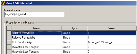
As you can see seen above, the Bulk Conductivity can be entered as a complex value with real and imaginary parts. In HFSS, to designate the imaginary part, multiply it by 1i, as shown above. The FSS looks as below with a substrate permittivity of 2.25:
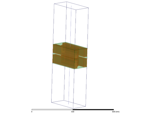
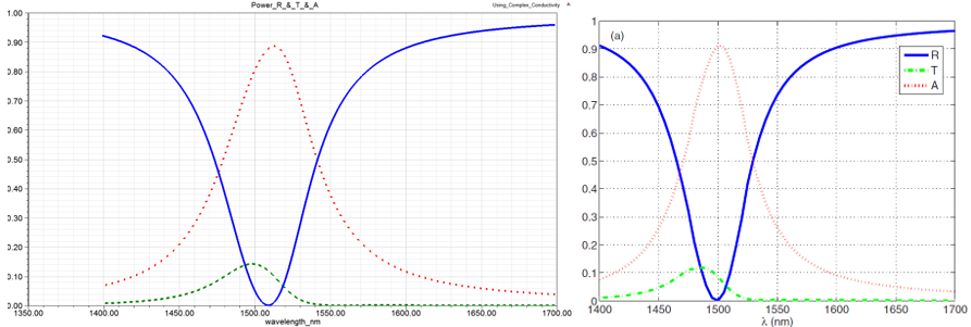
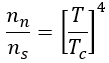
When solving this FSS with the complex conductivities in the short-wave-IR, from 1.35 um to 1.7 um, we get the traces shown below: Absorption (red dash), Reflection (blue), and Transmission (Green dash). The plot on the left is HFSS with the complex conductivity definition and the plot on the right is from the cited paper.
Generalized Superconductive Model
The generalized superconductive model treats a superconductor as a combination of classical electrons and Cooper pair, or superconducting, electrons. The classical electrons behave as in the Drude model contributing to loss while the Superconductive electrons behave entirely differently. The common model used to describe the dispersive electrical effects of a superconductor derives itself from this ‘2 body fluid’ model discriminating the electrons as such.
This model also represents the electrical effects of a superconductor with a complex conductivity that is a function of temperature and frequency. If the temperature is above the critical temperature, Tc, it will behave as the classical conductor, whether a semiconductor or metal. If the temperature is equal to or below the critical temperature, the behavior changes markedly to demonstrate many of the classical superconducting effects. For the 2 fluid superconductor model, the complex conductivity is as shown below:

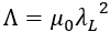
Note that the nn/ns ratio is the ratio of classical electrons to superconductive electrons and is a function of temperature:
 is a function of the London Penetration Depth,
Entry into HFSS just as we did for the Drude Model, using frequency dependent Project Variables as shown below:
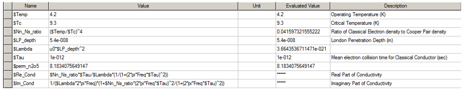
To demonstrate the accuracy of this model in HFSS, we comparison the literature for a Superconducting microstrip for the extraction of the propagation properties.2 A material was created representing the superconductor Nb in HFSS using a complex conductivity definition similar to the Drude Model. The temperature, T, of the Nb under test was 9.3K with a critical temperature, Tc, of 4.2K. The mean collision time was given as  sec.
sec.
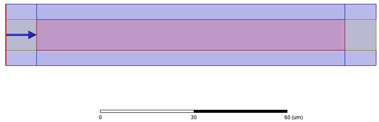
The microstrip is simulated by having a given length of line, in this case 100 um, and extracting the propagation constant from the phase of the insertion loss and the line length at 300GHz. Note that the port solver does not yet recognize complex conductivities so a PEC is used for the ground plane and trace at the waveport and de-embedded to the Superconducting Microstrip.
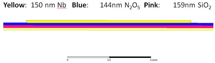
 = 54nm. The substrate is composed of 159 nm SIO2 under 144nm N2O5. The electrical properties used were:
  =6.25 &
With these dimensions the reference shows the following results for both a PEC signal and ground plane and the superconducting Nb trace and ground plane.
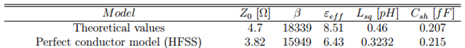
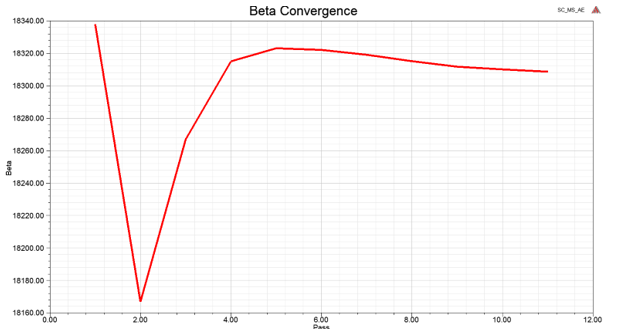
 for an automated accurate solution. HFSS converged to 18308.5 rad/sec with a 0.01% convergence criterion on
References
1) Avitzour, Yoav, et al. Wide-angle Infrared Absorber Based on a Negative-Index Plasmonic Metamaterial. Physical Review B 79, 045131. 2009.
2) Rafique, Raihan. Superconducting High Speed Passive Interconnects. A Dissertation from Chalmers University of technology, 2006