Helical Antenna

Abstract

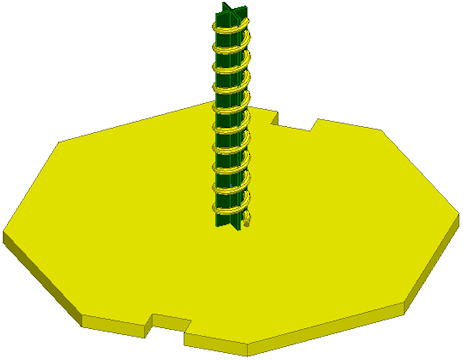
A coax-fed helical antenna with a dielectric support on a finite ground plane makes up the design.

The antenna is set up to run at 3.5 GHz. The design illustrates how to build a parametric helical antenna. Using Material override, geometries can overlap without error.

HFSS antenna example model, helical antenna with dielectric support on a finite ground plane

Version: 2024 R1

Description

Model Construction:

HFSS solution type: HFSS with Auto-Open Region Radiation selected
The support is made of Teflon and the ground has a thickness of 0.5 in. The coax port is internal and is capped by a conducting object. You can create a helix similar to this model by drawing a cross-sectional circle or polygon for the starting face and then clicking Draw > Helix while it is still selected. You must define two points for the axis direction of the helix as well as the pitch, number of turns, right/left hand, and optional radius change per turn.

Note:

To view a port or boundary, select the desired item in the Project Manager. It is then highlighted in the Modeler window, and the properties are displayed in the docked Properties window. Selecting an object in the History Tree will also display its properties.

Variables are used for the helix cross section, radius, number of turns, and more for future variation.

Under the radiation tab, multiple Far Field or Near Field setups are defined.

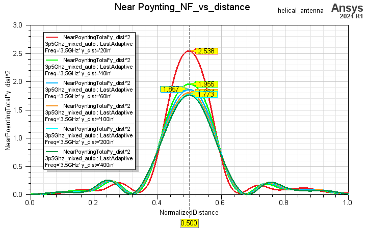
One post processing variable “y_dist” is defined to illustrate the variation of the radiated field from the Near Field to Far Field zone.

Excitations:

A wave port is defined internally so it will compute both the feed characteristic impedance and S parameters.

Setup:

Adaptive meshing is done at 3.5 Ghz - Convergence is set up to the default value (0.02).

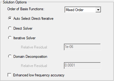
Solution Options are as follows:

Order of Basis Functions set to Mixed order, as the design contains a lot of small geometric details compared to wavelength. This setting can reduce the solution time.
Auto Select Direct/Iterative

solution options section under the options tab of the driven solution setup dialog box, showing specification of mixed order and auto select options

An interpolating sweep from 2.5 GHz to 4 GHz with 1001 points provides a smooth S parameters curve. Far fields, such as directivity or gain, are also computed for the frequencies directly included in the interpolating sweep. Specific frequencies can also be computed using a discrete sweep.

Simulation Time: 4 minutes (on a 6-core machine) – max RAM used 2GB

Postprocessing

Several plots have been defined and are listed in the Project Manager under Results. Double-click any of them to see the plot. The plots are shown below, organized according to the type of report.

far fields reports

The following far fields reports have been predefined:

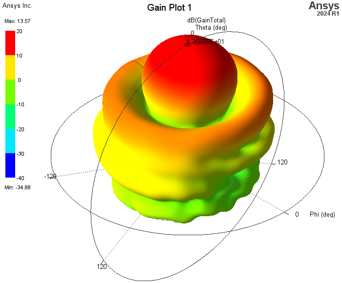
3D Polar Plot of Total Gain in Decibels:

3D polar plot of total gain in decibels

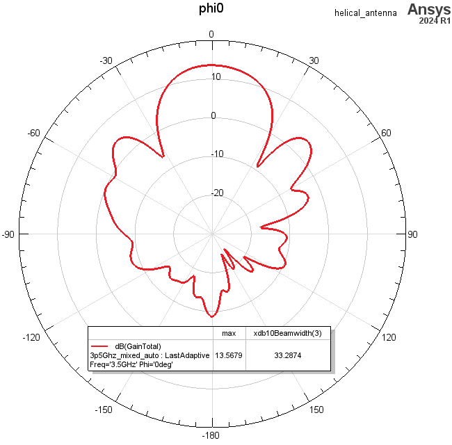
2D Polar Plot of Total Gain in Decibels for phi = 0°:

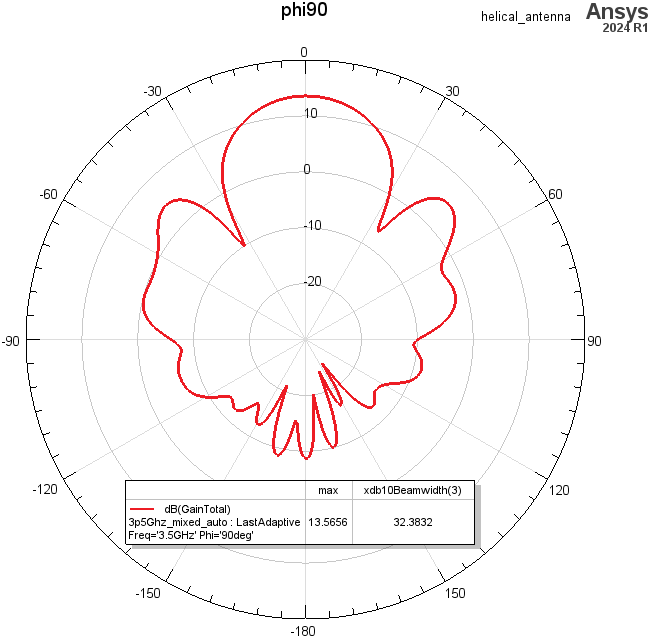
2D polar plot of total gain in decibels for angle phi equals zero degrees

2D Polar Plot of Total Gain in Decibels for phi = 90°:

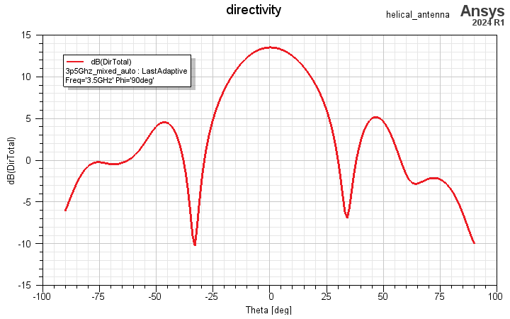
2D polar plot of total gain in decibels for angle phi equals ninety degrees

Total Directivity in Decibels vs. Theta:

total directivity plot in decibels versus angle theta

modal solution data reports

The following modal solution data report has been predefined:

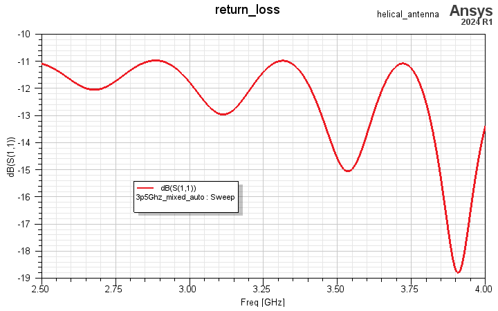
S Parameter_1,1 – Return Loss vs. Frequency:

S parameter plot, return loss versus frequency

antenna parameters reports

The following antenna parameters report has been predefined:

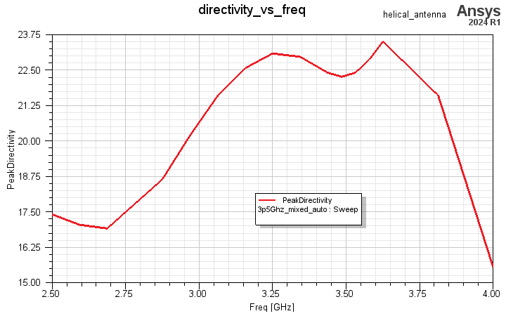
Peak Directivity vs. Frequency:

peak directivity versus frequency plot

near fields reports

The following near fields reports have been predefined:

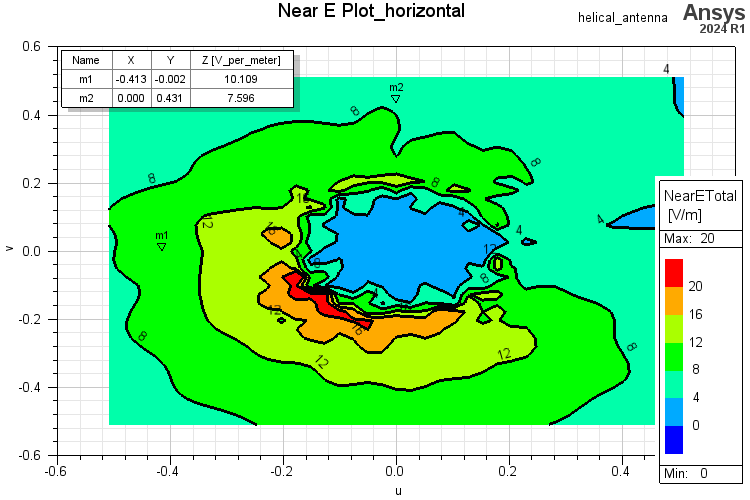
Near E_Total, 2D Contour Plot, Horizontal Cut (based on the horizontal_near_field radiation setup):

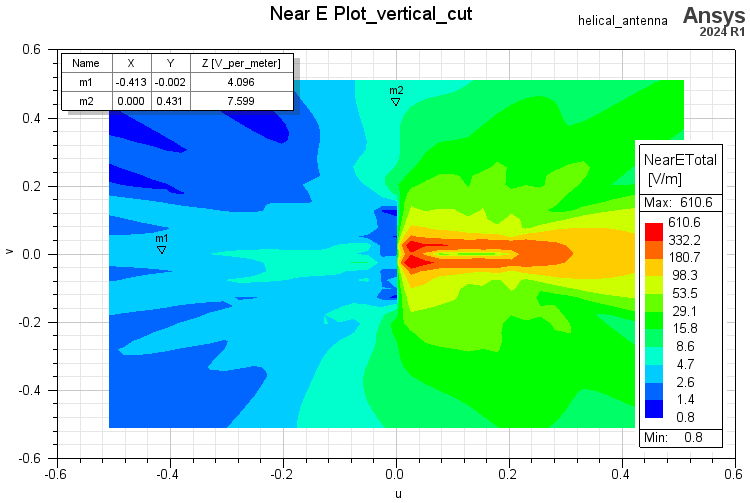
near E total 2D contour plot along horizontal cut plane

Near E_Total, 2D Contour Plot, Vertical Cut (based on the vertical_near_field radiation setup):

near E total 2D contour plot along vertical cut plane

Magnitude of Poynting vs. Distance (“y_dist” variable) – illustrating Near Field / Far Field Zone:

magnitude of poynting versus normalized distance, illustrating near field slash far field zone

You can add markers to any of the plots by right-clicking on the plot window and choosing Marker > Add Marker, Add X Marker, or Add Y Marker.

To overlay the 3D gain plot on the model, click HFSS > Fields > Plot Fields > Radiation Field to display the Overlay radiation field dialog box. Check Visible for 3D Polar Plot 1 and set the transparency and scale as desired:

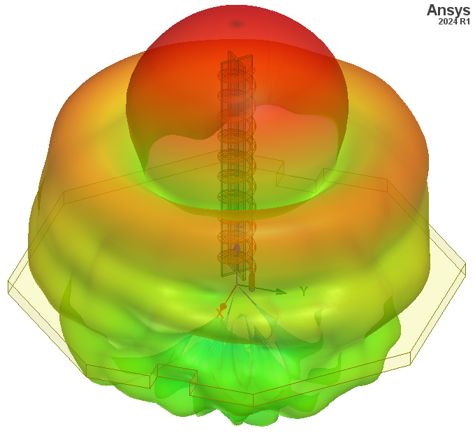
3D polar plot 1 overlaid on the model geometry

Similarly, here is the appearance when the Near E-Plot_vertical_cut and Near E-Plot_horizontal fields are overlaid on the model:

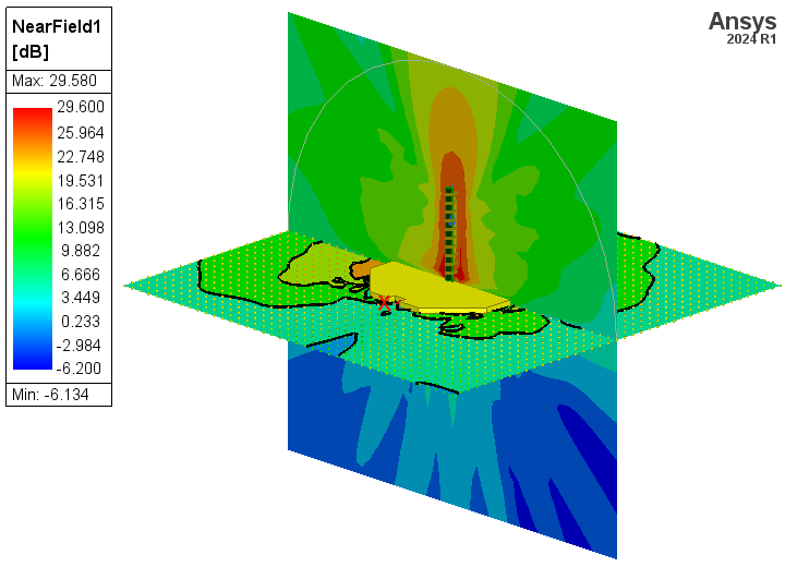
2D contours, near E horizontal and near E vertical, overlaid on model geometry

Add the legend by right-clicking Field Overlays in the Project Manager and choosing Plot Sampled Near Field from the shortcut menu. Finally, choose the Near ETotal and dB options.