Differential Pair Microstrip

The differential microstrip design comprises two copper traces and an FR4 substrate enclosed in an air-box. The design in the following figure describes an efficient way to model a long transmission line without explicitly drawing the desired length of the microstrip model. HFSS offers a post processing feature called Deembedding that can be used to calculate the transmission line characteristics by moving the reference plane of the wave port by the specified deembedding distance.

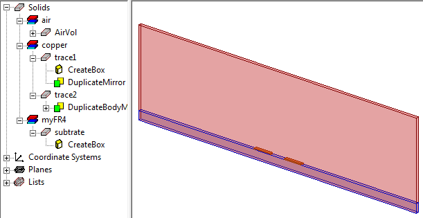
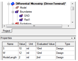
Differential microstrip and project tree panel.

The dimensions of the copper traces, air-box, and substrate are defined by using variables. If you click the design name on the Project Manager window, the Properties window displays all the design variables.

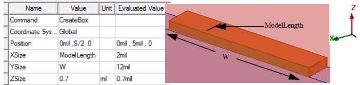
Properties panel displayed in the project manager window.

Double-click CreateBox under trace1 on the history tree to see the dimensions of the copper trace.

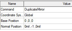
Table with dimensions. Coppper trace model.

In this model, trace2 was created from trace1 by right-clicking trace1 and selecting Edit > Duplicate > Mirror. In the coordinate text boxes of the status bar, starting co-ordinates for the base position was set to 0, 0, 0 and the normal position was set to 0,-1,0.

Coordinate group box displaying coordinate system.

By parameterizing with common variables and taking advantage of the model tree you can create efficient designs in HFSS. Changing the value of one or more common variables ensures individual objects to track with the geometry of the entire model appropriately.

Boundaries and Excitations

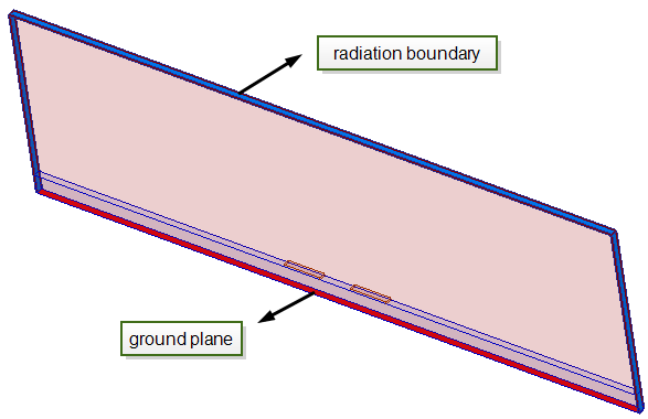
On the Project Manager window, click GND and Rad1 to see the ground assigned on the bottom face of this design, and the radiation boundary assigned on the top face and along the ZX faces as shown in the following figure.

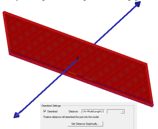
Note: You can also select the Boundary Display (Solver View) option from the HFSS menu item and select the boundaries, ports, and terminals that you want to see in the design. In the following figure, the ground and the radiation boundary appear highlighted since they are selected on the Boundary Display (Solver View) dialog box.

Model with ground and radiation boundary highlighted.

Observe how the two ports are assigned in the remaining faces in the following figure.

Model with deembed groupbox and port face orientations.

Note:

For guidelines on defining port size, see the section Assign Wave Ports for Terminal Solutions in the help.

The ports are deembedded with a negative distance outwards from the structure. The intent is to solve the model of this minimal length and then deembed outwards from the ports using a negative sign for the deembed distance to effectively add the extra length that you want to represent the actual length of the model.

Note:

For more information about modeling long transmission lines, see the Applications for Deembedding section in the Assign Excitation material in the help.

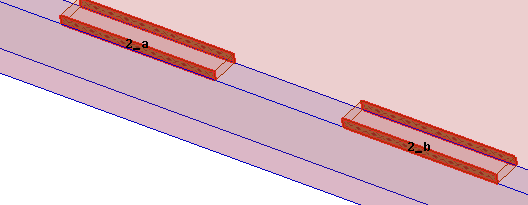
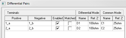
There are 4 terminals assigned as shown in the following figure.

Right-click Excitations and select Differential Pairs to access the Differential Pairs dialog box.

HPC Analysis and Solution Setups

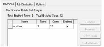
Run this design at an adapt frequency of 20 GHz. Since a parametric sweep (look for SpacingSweep under Optimetrics on the Project Manager window) is defined, this design is a good choice for which HPC can be set up. On the Solution Setup dialog box, click the button to open the HPC and Analysis Options window. Click Add and set the number of tasks and cores.

For example in HPC setup in the following figure, the design was simulated on a machine with 12 cores on it and the Number of Tasks is 3. In such a setup, 3 frequency points are solved in parallel with 4 cores of matrix multiprocessing per frequency point.

Machines for Distributed Analysis group box.

Note:

For more information about HPC, see HPC and Analysis Configuration Options section in the help.

While deembedding simplifies modeling long differential striplines and makes the solution process efficient, the HPC setup further accelerates the simulation process.

Results

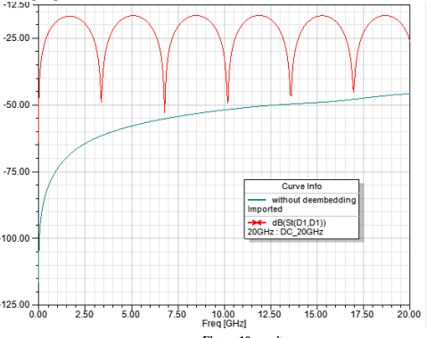
The results of the S-parameter plots with and without deembedding are shown below. The deembedding operation adds the effect of phase delay and additional dielectric and conduction losses to the resulting S-parameter calculated from this model.