
Coaxial Resonator
Description - A coaxial resonator model showing how to use the Eigenmode solver. The eigen solver computes the resonant frequency and Q of the model. This example was taken from Microwave Circuit Modeling Using Electromagnetic Field Simulation (D. Swanson Jr., W. Hoefer).
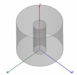
Model - A coaxial cavity. Walls are defined to have s = 6.17 x 10⁷ mho/m.
Setup - There are no defined sources in an eigen solution so you need only select the number of modes to compute and the convergence criteria. For this model, only the first mode is computed. For maximum accuracy, we need to use curvilinear elements. To verify that this has been set for the model, go to HFSS > Mesh > Initial Mesh Settings, and make sure “Apply Curvilinear Elements” is checked.
Selecting an object in the History tree will also display its properties.
Coaxial Resonator Post Processing
After solving, you can view solution data by right-clicking on Setup1 and selecting Eigenmode Data to display the Solution dialog. You also view the Solution tabs for Profile, Convergence, and Mesh Statistics.
To view the resonant frequency and Q, select the Eigenmode Data tab on the Solution dialog.*
To view the shade plot, right-click E Field under Field Overlays in the Project tree, and select Update Plots.
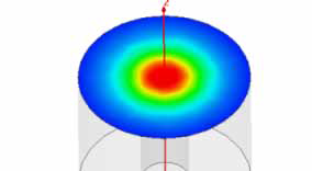
* Data computed using a mode matching program are given in the reference. The results presented are f0 = 1.87 GHz and Q = 5592.