Related Topics:

Causality Constraints on the Impulse Response

Causality Constraints on the Frequency Response

The Hilbert Transform Test for Causality

The Generalized Hilbert Transform Test for Causality

Truncation and Discretization Errors in Causality Testing

Accounting for the Truncation Error

Accounting for the Discretization Error

The Causality Test with Minimized Errors

Fixing the Values for the Total Error Bound

Examples of Truncation Error Formulas

Causality Constraints on the Impulse Response

Consider a system with impulse response h(t) that is excited by a signal x(t), producing an output y(t). For an LTI system, these quantities are related through the convolution integral:

(1)

where the operator (*) denotes a linear convolution.

A causal system must be nonanticipatory, that is, y(t) from equation (1) should depend on x(t) for t <= t. Restating this requirement, a time domain signal h(t) is causal if:

(2)

By equation (2), a causal h(t) is sufficient to ensure that y(t) does not precede x(t). It can be shown that a causal h(t) is both necessary and sufficient.

Causality Constraints on the Frequency Response

The frequency-domain response H(jw) is the Fourier transform of time-domain signal h(t):

(3)

where F{} denotes the Fourier transform, j² = -1, and w is the angular frequency.

The constraints on a causal frequency response can be derived as follows. A causal h(t) satisfies the condition:

(4)

where the function sign(t) returns 1 for t>0, 0 for t=0, and -1 for t<0.

Taking the Fourier transform of equation (4), to obtain:

(5)

where F{} denotes the Fourier transform, * represents convolution, and the integral is defined according to the Cauchy’s principal value (p.v.) to avoid the singularity. The rightmost side (RHS) of equation (5) is known as the Hilbert transform of H(jw).

The Hilbert Transform Test for Causality

The Hilbert transform is the basis for causality testing and enforcement. Here is a brief derivation.

Let R₀ denote the operator in the RHS of (5):

(6)

Then from equation (5) a causal frequency response is invariant (maps onto itself) under the operator R₀:

(7)

The causality test uses an equivalent formulation. A frequency response H(jw) can be separated into its real and imaginary parts:

(8)

From equation (8), the real and imaginary parts of a causal H(jw) are Hilbert transforms of each other. If a frequency response satisfies this constraint, it is declared causal.

The Generalized Hilbert Transform Test for Causality

The conditions in (6) are sufficient for causality, but are not necessary. In particular, the constraints in (6) are true only for a response H(jw) that is square-integrable. The function H(jw) is square-integrable if:

(9)

The constraints in (6) have been shown to be necessary and sufficient conditions for causality with square-integrable functions (See Causality Reference [3]). An example of a square-integrable function is the driving-point impedance of a parallel RC circuit:

where G=1/R and C are positive real constants.

Here are example functions that are not square-integrable (R, L, and C are positive real constants). These functions are causal but do not satisfy (6):

For functions that are not square-integrable, the necessary and sufficient conditions for causality are given by the generalized Hilbert transform (See Causality Reference [3]). The generalized Hilbert transform of H(jw), H_n(jw), is given by:

(10)

where n is the number of subtraction points, and

represents the subtraction points spread over the available bandwidth W (See Truncation and Discretization Errors in Causality Testing for details on bandwidth W).

L_H(jw) is the Lagrangian interpolation polynomial for H(jw) (See Causality Reference [6]):

(11)

The Hilbert transform in (6) is a special case of the Generalized Hilbert transform when n=0, hence the term “Generalized.” From equations (10) and (11), if n = 0 then L_H(jw) = 0, and the P terms in (10) disappear. The resulting equation is the Hilbert transform of H(jw), equation (6).

Let R_n denote the reconstruction operator in the RHS of (10):

(12)

Then a causal frequency response, square-integrable or not, maps onto itself under R_n:

(13)

Equation (13) can be used to test whether or not a frequency response is causal. A causal frequency response maps onto itself under the operator R_n, but a noncausal response does not.

If a frequency response is causal, all its network transforms are also causal. That is, if H(jw) is a scattering parameter and is causal, the corresponding impedance and admittance parameters are causal.

Truncation and Discretization Errors in Causality Testing

Causality of a frequency response can be tested by verifying whether or not the frequency response satisfies (13): a causal response is equal to its reconstruction via the generalized Hilbert transform (GHT). If the frequency response is noncausal, then it does not equal its own GHT reconstruction. In a physical computation, two quantities are deemed “equal” when the difference between them is not greater than a minimum tolerance set by the computing hardware. In addition to the hardware tolerance, the causality test must also account for any errors inherent in the calculations themselves.

Significantly, the test in (13) is valid only when H(jw) is known continuously for all frequencies:

By contrast, frequency responses in the form of Touchstone data is known only at discrete frequencies in a finite bandwidth:

where w_max is the maximum available angular frequency in the data.

One possibility is to use the test in (13), but limit the integral in (12) to W, ignoring the contributions of the out-of-band integral, and interpolate H(jw) within W, so (12) can be computed. However, this attempt at reconstruction of a frequency response using the GHT is subject to two types of errors:

• The truncation error due to omitting the response at frequencies outside the bandwidth of the given data.
• The discretization error due to approximating a continuous response on the sampled (discrete) frequency data.

The unreliability that results on these two errors can lead one to falsely declare a causal response as noncausal (false positive) or a noncausal response as causal (false negative). A reliable test for the causality of tabulated data must account for both truncation and discretization errors.

Accounting for the Truncation Error

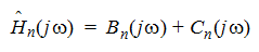
To compensate for the missing out-of-band data, the following formulas can be applied. Separate the reconstructed frequency response (12) into in-band [B_n(jw)] and out-of-band [B'_n(jw)] contributions.

(14)

The in-band contribution to the frequency response is:

(15)

See Accounting for the Discretization Error to continue to read about evaluation of the in-band contribution.

Evaluating the out-of-band contribution to H(jw) involves integrating over the frequencies in W^C, the frequencies that are outside of W:

(16)

The Cauchy’s integral in this term can be replaced by a regular integral, since the integrand does not have a singularity for w' = w in W^C. Further separate this modified integral for the out-of band response to reflect the separate contributions from H(jw) and L_H(jw).

(17)

C_n(jw) is the integration term for L_H(jw):

(18)

Since L_H is an nth-order polynomial, a closed-form expression for C_n(jw) can be derived.

The integration term for H(jw) is -E_n(jw). This is the truncation error.

(19)

Since H(jw) is not defined outside W, E_n(jw) cannot be evaluated directly. However, the error introduced by omitting this term can be quantified by fixing the behavior of H(jw) in W^C. If:

(20)

where M is a real constant, , a = 1, 2, 3..., then it can be shown that a bound for the truncation error exists such that:

(21)

where T_n(w), the truncation error bound, is defined as:

(22)

The bound in (21) has been shown to be tight (See Causality Reference [5]). Due to its Lagrange-polynomial nature, T_n(w) is bounded only for frequencies:

(23)

where e is a small number (<0.1).

This bound can be made arbitrarily small by increasing the number of subtraction points, n. It can be shown from (22) that T_n(w) decreases as n increases. From (21), when T_n(w) is reduced, the truncation error is correspondingly reduced.

Thus, the disadvantage of not knowing the frequency response outside of the bandwidth (e.g., in W^C) can be offset by increasing the number of subtraction points, n, in the computation of H_n(jw). This ability to control the truncation error with subtraction points is a second reason to use the GHT rather than the simple Hilbert transform, especially for data with limited bandwidth.

The approximation to H_n(jw) can omit the E_n(jw) term while increasing n such that T_n(w) is kept smaller than a user-specified tolerance. The truncated approximation to H_n(jw) becomes:

(24)

Accounting for the Discretization Error

The discretization error occurs in the evaluation of the in-band contribution, B_n(jw):

(25)

An evaluation of the in-band contribution has two aspects: (1) the approximation to the integral and (2) the interpolations involving the sample frequencies w_k and the subtraction frequencies w_q. Errors in each of these aspects contributes to the discretization error.

If is the approximation to , the error in this approximation, D_n(jw), is:

(26)

The bound for the discretization error is obtained by subtracting the estimates computed using two different combinations of integration rules and interpolation methods, and is given by:

Where m1 and m2 are two different interpolation methods and n1 and n2 are two different integration rules. The discretization error is reduced if the bound is reduced. The truncation error bound can be reduced by increasing the number of frequency points in the tabulated data.

The Causality options s_element.interpolation_typecc and s_element.integration_typecc control the mix of interpolation and integration methods to be applied in the evaluation of the in-band data and the calculation of the discretization error bound.

Interpolation and Integration in Causality Checking

Interpolation Type	Integration Type	m1	m2	n1	n2
Spline	Numerical	Cubic Spline	PCHIP	Simpson’s Rule	Trapezoidal Rule
Spline	Analytical	Cubic Spline	PCHIP	N/A	N/A
Rational Function	Numerical	RF1	RF2	Simpson’s Rule	Trapezoidal Rule
Rational Function	Analytical	RF1	RF2	N/A	N/A

The interpolation between frequency points can use Splines or Rational Functions. When Spline interpolation is chosen, the interpolation is performed using cubic splines. In the calculation of the discretization error bound, the interpolation methods m1 and m2 are the cubic spline and the piecewise cubic Hermite interpolation polynomial (PCHIP), respectively. When interpolation by Rational functions is chosen, m1 and m2 are two different rational function approximations with different approximation errors.

The integration terms can be evaluated numerically or analytically. If Numerical integration is chosen, the two integration rules n1 and n2 are Simpson’s method and the Trapezoidal rule, respectively. When Analytical integration is chosen, n1 and n2 are the same, and do not contribute to the estimate of the discretization error. With analytical integration, only the interpolation methods m1 and m2 affect the discretization error bound.

See Understanding the Causality Options for more information on these options.

The Causality Test with Minimized Errors

Now construct a causality test that minimizes both truncation and discretization errors.

(27)

For a causal frequency response, the ideal reconstruction error is “zero”, subject to the computational limit of the hardware.

The numerical reconstruction error equals the ideal reconstruction error plus the truncation and discretization errors:

Therefore, the numerical reconstruction error satisfies the following inequality for any H(jw).

(28)

If and only if H(jw) is causal, the reconstruction error vanishes at all frequencies.

(29)

For a causal signal, the reconstruction error never exceeds the total error bound:

(30)

When this condition is met, any causality violations in H(jw) are too small to be flagged, and the data can be declared causal. If the reconstruction error exceeds the threshold at any frequency:

(31)

then H(jw) can be declared to be noncausal.

Since the overall objective is to satisfy the fitting error d_fit (See Fixing the Values for the Total Error Bound), equations (30) and (31) are too stringent. The data can fail the test in (31) and be declared noncausal, yet still produce an acceptably low fitting error. Thus, equation (31) can be modified, as follows:

(32)

When this condition is met, any causality violations in H(jw) are too small to affect the fitting error, and the data can be declared causal.

If the reconstruction error exceeds the fitting error threshold at any frequency:

(33)

then H(jw) can be declared to be noncausal.

Fixing the Values for the Total Error Bound

Since T_n varies with n, the total error bound must also vary with n. Also, since varies with the frequency steps in the tabulated data, must also vary with frequency step. It is important to set to reasonable values. Very large values for can hide causality violations, while very small values can flag any response as noncausal.

The following strategy assigns reasonable values to . Typically, the maximum tolerable magnitude of noncausality, , is known a priori.

In previous versions, Nexxim set to 10^-4 (0.01%), and the value could not be changed by the user. Experimentation showed, however, that a tolerance of 0.01% was too conservative: macromodels with acceptable fitting errors are flagged as noncausal. Since the success of the macromodel fitting process is the ultimate goal, the causality tolerance d_nc was set equal to the tolerance for the fitting error, d_fit, which was 1%. Even this choice for the causality tolerance was found to be conservative, and could be increased. The current setting for the tolerance for the fitting error, d_fit has been reduced to 0.5% (to produce more accurate fits, while the default causality tolerance has been set to five times the default tolerance for the fitting error d_fitor 2.5%.

(34)

If the value of d_nc is set by the user (with the option causality_check_tolerance), then that value is used and the relationship in equation (34) is not considered.

The earlier causality checker tolerance of 1% was found to produce a high number of inconclusive cells. Here is the plot for a 56-port Touchstone file with a causality error tolerance of 1%. Note the yellow cells indicating inconclusive results, and the red cells indicating causality violations, which may include false positives.

Despite these results, the data can be fitted to a state-space model with a fitting error of less than 0.5%.

Here is the plot for the same 56-port Touchstone file with the current 2.5% causality tolerance (and some causality checker improvements). Note that all cells are conclusive now.

Once the tolerance for noncausality d_nc has been determined, a reasonable n is chosen in the evaluation of the GHT such that the truncation error is always less than the tolerance by a fixed proportion:

(35)

(36)

where . Based on experimentation, Nexxim sets e to 0.05.

When the frequency steps in the tabulated data is small, the discretization error bound is much smaller than the truncation error bound. When the discretization error is small:

(37)

the total bound follows T_n(w) very closely. As a result, when T_n satisfies (33), the total error bound often also satisfies (33), that is:

(38)

In this situation, the test described here has sufficient resolution to detect causality violations with magnitude greater than . If the frequency steps in the tabulated data is not small, can be comparable in magnitude to T_n(w). In this case, can be greater than . When this condition is detected, the best solution is to reduce the maximum frequency step in the tabulated data and repeat the causality test until satisfies (34).

Examples of Truncation Error Formulas

Here are some graphic examples of the truncation error formulas. NOTE: These internally computed values are not available for plotting in Electronics Desktop.

Figure 1. Truncation error T_n(w) decreases with the number of subtraction points, n.

In Figure 1, the truncation error bound T_n(w) from (18) is compared over different values of n for a scattering parameter is known up to 10GHz. For an S-parameter, M=1 and a=0 in (16) and (18). In Figure 1, T_n(w) has a local minimum at each subtraction frequency . Since T_n(w) is shown only for non-negative frequencies, only half the number of subtraction points are plotted.

In Figure 2, T_n(w) is shown for various values of d_nc. As d_nc is reduced from 0.01 to 0.0001, Nexxim increases the number of subtraction points n from 10 to 22, so for .