


The Motion solver supports static, dynamic, thermal, and eigenvalue analysis for the system and body eigenvalue analysis for a nodal FE body and nodal EasyFlex body.
When the Motion Solver is running, analysis generally proceeds in the following order.
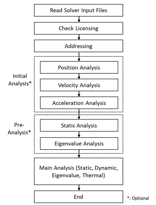
- Read Solver Input Files
At this stage, the solver reads the input files, such as DFS, SSC, GINF, and DFMF, which contain all the necessary information about the mechanical system to be analyzed. These files include model information, simulation scenarios, and modal data.
- Check Licensing
Following the input files, the solver checks for the appropriate licensing. If the license is invalid, analysis will stop. Ansys Motion requires a base license, known as the vmotion license feature, to operate. Depending on the complexity and specific requirements of the model, additional licenses may be needed. For instance, models incorporating Drivetrain components require the vmotion_toolkit license feature. Academic licenses may have restrictions based on model degrees of freedom, such as the number of nodes. Detailed information on licensing requirements can be found in the academic license documentation.
- Addressing
The addressing step is pivotal in organizing the data or variables necessary for analysis. Here, the solver constructs the required data structures and allocates memory. It preprocesses the data read from the input files, calculating necessary values for the analysis. Examples include processing geometric data like patch areas and edge lengths, initializing of the user subroutine functions, and identifying relationships between generalized coordinates and applied forces.
- Initial Analysis (if required)
The initial analysis is utilized to establish the starting positions and orientations of bodies due to motion constraints or the initial conditions of joints, aiming to identify the positions and orientations of bodies that minimize constraint violations. This phase includes calculating the initial velocity of a body by considering its kinematic relationship with other bodies and finding the body's initial acceleration that satisfies the equations of motion. Initial analysis can be conducted as an independent process or serve as a preparatory step for dynamic analysis, depending on the selected analysis type.
- Pre-Analysis (if required)
If the analysis type is set to dynamic analysis, pre-analysis may be conducted based on the analysis settings. When the inclusion of static analysis is activated in the analysis settings, the solver seeks a static equilibrium state based on the initial conditions provided. Dynamic analysis then commences from this state of static equilibrium. Alternatively, if the inclusion of eigenvalue analysis is activated in the analysis settings, eigenvalue analysis of the initial state can be performed.
- Main Analysis
The solver executes the selected type of analysis, whether it is Static, Dynamic, Eigenvalue, or Thermal.
- End of Analysis
After analyzing the data, the solver assesses the resources used, including memory and CPU, and outputs the results, including performance metrics, in a message file (msg), indicating the end of the simulation process. The solver frees all memory and closes all open files.
The initial analysis determines the starting positions and orientations of bodies in a multibody dynamic system, guided by motion constraints or joint initial conditions. Its purpose is to identify body configurations that minimize constraint violations, laying the groundwork for further analysis. This includes calculating initial body velocities, taking into account kinematic relationships, and determining initial accelerations that adhere to the equations of motion. The analysis can be used alone or as a preliminary stage for dynamic analysis. The initial analysis is performed in a specific order: position, velocity, and acceleration analysis. Each analysis can be omitted if not desired.
Position analysis focuses on solving for the positions and orientations of bodies in a system that minimize constraint violations at the positional level. Initial conditions at the position level are treated as constraints in position analysis. This phase omits the consideration of external and internal loads, focusing solely on geometric and kinematic constraints and initial conditions at the position level. It assumes that flexible bodies, such as FE bodies and EasyFlex bodies, are rigid.
The solver adjusts the body's position and orientation to meet constraints in cases such as:
If the reference or mobile coordinate system of a joint is set to a position and orientation that prevents relative movement.
If an initial positional condition is specified through the joint's motion or initial condition.
If position analysis is skipped, velocity analysis starts from the initial position and orientation. Should there be any constraint violations, significant constraint forces might be generated to satisfy these conditions as dynamic analysis begins. This situation can cause failures during the Newton-Raphson process, requiring careful consideration to avoid such outcomes.
Governing Equations for Position Analysis
The governing equations for position analysis can be written:
 | (9–1) |
 | (9–2) |
where:
| q = generalized coordinates |
| Δq = change of the generalized coordinates during the NR (Newton Raphson) iteration |
| M = mass matrix of the system |
| Φ = constraint equations at the position level |
| Φq = partial derivatives of the constraint equations at the position level with respect to the generalized coordinates. |
| λ = Lagrange multiplier |
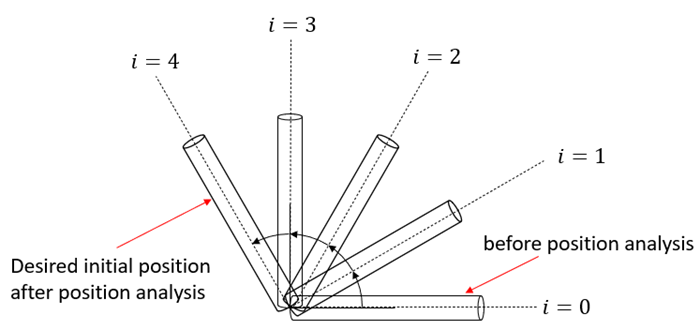
Global iterations in Position Analysis refers to the iterative process used to improve the initial position estimation of the joints and bodies in a multibody system under motion constraints or initial conditions. One global iteration means repeating the entire position analysis process once. By default, a global iteration is one, but if the initial conditions are large and convergence is difficult, multiple global iterations can be performed to gradually approximate the initial conditions. This technique is particularly useful when dealing with large initial conditions that impede rapid convergence using standard methods like Newton-Raphson due to their local convergence properties. The iterative process involves performing the position analysis multiple times, incrementally adjusting the large initial condition values.
To illustrate, if the initial angle due to certain motion constraints is 120 degrees and the global iteration number is set to 4 in the analysis settings, the initial conditions in each iteration would be 30 degrees, 60 degrees, 90 degrees, and finally 120 degrees. This approach allows the system to converge more smoothly by gradually approaching the final condition.
The equations used in the global iterations are:
 | (9–3) |
 | (9–4) |
where:
| DΦi = driving constraint equations for i-th global iteration in the position level |
| qba = relative translational displacement (sba) or relative angular displacement (θba) between action and base markers with respect to the base marker |
| F = motion function (user-defined) |
| q0 = initial condition in the position level (user-defined) |
| i = current global iteration count |
| Npos = total number of global iterations as defined as Number of Steps in Initial Position Analysis setting in the analysis settings. |
Velocity analysis focuses on solving for the velocities of bodies in a system to minimize constraint violations at the velocity level. Initial conditions at the velocity level are treated as constraints in velocity analysis. This phase omits the consideration of external and internal loads, focusing solely on geometric and kinematic constraints and initial conditions at the velocity level. It assumes that flexible bodies, such as FE bodies and EasyFlex bodies, are rigid.
The solver adjusts the body's velocities to meet constraints in cases such as:
If the reference or mobile coordinate system of a joint is set to velocities that prevent relative movement.
If an initial velocity condition is specified through the joint's motion or initial condition.
If velocity analysis is skipped, dynamic analysis starts from the initial velocities. Should there be any constraint violations, significant constraint forces might be generated to satisfy these conditions as dynamic analysis begins. This situation can cause failures during the Newton-Raphson process, requiring careful consideration to avoid such outcomes.
Governing Equations for Velocity Analysis
The governing equations for velocity analysis can be written:
 | (9–5) |
 | (9–6) |
where:
 = time derivative of generalized coordinates = time derivative of generalized coordinates |
 = change of the time derivative of generalized coordinates
in the NR (Newton Raphson) iteration = change of the time derivative of generalized coordinates
in the NR (Newton Raphson) iteration |
 = mass matrix of the system = mass matrix of the system |
 = constraint equations at the velocity level = constraint equations at the velocity level |
 = partial derivatives of the constraint equations at the
velocity level with respect to the time derivatives of generalized
coordinates. = partial derivatives of the constraint equations at the
velocity level with respect to the time derivatives of generalized
coordinates. |
 = Lagrange multiplier = Lagrange multiplier |
Acceleration analysis focuses on solving for the accelerations of bodies in a system to satisfy the constraint equations at the acceleration level and equations of motion. Unlike position and velocity analysis, in acceleration analysis, all load conditions are considered, and flexible bodies are not treated as rigid, so nodal accelerations are taken into account.
If acceleration analysis is skipped, next process starts from the zero accelerations. After skipping acceleration analysis, if dynamic analysis follows, the initial acceleration error can be larger when dynamic analysis starts. In this case, the initial time step size should be set to a smaller value than the default. For example, an initial time step size of 1.0e-6 is preferable to the default value of 1.0e-4.
Governing Equations for Acceleration Analysis
The governing equations for acceleration analysis can be written:
 | (9–7) |
 | (9–8) |
Static analysis is a fundamental approach to understanding the behavior of mechanical systems under steady state conditions. This method focuses on calculating the static equilibrium position and the forces acting on a system, taking into account any non-linear effects that may be present. The Motion solver supports three types of static analysis: linear without a rigid mode, nonlinear with a rigid mode, and nonlinear without a rigid mode. The selection of the appropriate type depends on the specific characteristics of the system being studied and the nature of the properties involved.
Linear Static Analysis without a Rigid Mode
Linear static analysis without rigid modes is typically used for systems fixed to the ground with joints or stiffness, preventing any rigid movement between parts. This method is most effective when the system components have only linear properties and there is no need to account for rigid body modes. This is especially helpful in situations where a precise and straightforward analysis of structural equilibrium is necessary, without the added complexities of rigid body movements, large deformation, or non-linear behaviors.
The governing equation for this form of analysis is represented as:
 | (9–9) |
 | (9–10) |
where:
| Φq = partial derivatives of the constraint equations at the position level with respect to the generalized coordinates |
| λ = Lagrange multiplier |
| Q = generalized forces |
| Φ = constraint equations at the position level |
| q = generalized coordinates |
Non-Linear Static Analysis with a Rigid Mode
Non-linear static analysis with a rigid mode is necessary for systems that exhibit non-linear behavior or allow rigid body modes. This method makes it suitable for a broader range of applications, accommodating non-linearities and contact interactions effectively.
The analysis involves two main steps to find the static equilibrium position. Firstly, use the Newton-Raphson method to find a local solution while satisfying the governing equation:
 | (9–11) |
 | (9–12) |
The second step is to find a global solution while minimizing the position change
in the equations above. The solver repeats the entire Newton-Raphson process until
the delta velocity ( ) approaches zero. If the delta velocity does not approach zero
after finding the local solution, the solver resets the velocity and acceleration of
the system to zero and proceeds to the next Newton-Raphson step. When the delta
velocity approaches zero, it is considered that the global solution has been
reached, and the position at this point is regarded as the final static equilibrium
position.
) approaches zero. If the delta velocity does not approach zero
after finding the local solution, the solver resets the velocity and acceleration of
the system to zero and proceeds to the next Newton-Raphson step. When the delta
velocity approaches zero, it is considered that the global solution has been
reached, and the position at this point is regarded as the final static equilibrium
position.
Non-Linear Static Analysis without a Rigid Mode
Non-linear static analysis without a rigid mode is especially useful for evaluating structural systems that contain non-linear materials or undergo large deformations. If the system has no rigid body motion and exhibits nonlinear characteristics, such as displacement-stiffness or velocity-damping curves, this option can be beneficial. However, its usefulness decreases when dealing with systems that involve rigid body movements or contact dynamics. The governing equation is the same as that for Linear Static Analysis without a Rigid Mode (Equation 10.9 ~ 10.10) but uses the Newton-Raphson method to find a solution while satisfying the governing equation.
Remarks
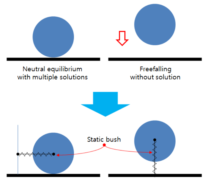
Since the mass matrix is used to avoid a singular problem in Equation 10.11, this analysis is numerically stable for a system in which bodies or nodes have a non-zero mass.
For neutral equilibrium, unstable or a free-falling problem as shown in the figure above, static bush force can be useful to avoid this problem.
Most contact problems are typical examples of an unstable static problem because of zero stiffness in the tangential direction at the contact point. When contact does not occur, the governing equation has zero stiffness for the contact normal direction. For these cases, it is difficult to find the static position in static analysis. It is better to use dynamic analysis to find the steady state solution.
Dynamic analysis is used for examining the behavior of mechanical systems in motion within the time domain. It goes beyond static analysis by considering the movement and forces acting on bodies dynamically. Dynamic analysis offers insights into a system's performance under motion, taking into account all nonlinear effects, including material nonlinearity, geometric nonlinear effects, and changes in boundary conditions due to dynamic events such as contacts and variable external loads.
The governing equations for dynamic analysis include inertia, damping, spring, and constrained forces, providing a comprehensive model of the system dynamics. The general form of the equations of motion is given by:
 | (9–13) |
 | (9–14) |
where:
| M = mass matrix of the system |
| q = generalized coordinates |
 = second time derivatives of the generalized coordinates = second time derivatives of the generalized coordinates |
| Q = generalized forces |
| Φ = constraint equations at the position level |
| Φq = partial derivatives of the constraint equations at the position level with respect to the generalized coordinates |
| λ = Lagrange multiplier |
During the time integration process, the velocity and acceleration are corrected to satisfy the formulas below to satisfy the velocity and acceleration constraints.
 | (9–15) |
 | (9–16) |
The Motion solver integrates variables in the time domain using the generalized α method (Chung and Hulbert ([1]), which is an implicit time integration method. The integration formula is as follows:
 | (9–17) |
 | (9–18) |
Kinematics analysis is automatically carried out when the degrees of freedom of the system is zero.
where:
 | (9–19) |
 = time derivatives of the generalized coordinates = time derivatives of the generalized coordinates |
| Δt = time step size |
| γ and β = Newmark's integration parameters |
| ρ∞ = spectral radius for infinite time step |
| n = numerical damping parameter (user input value) |
| i = current step |
| i+1 = next step |
The motion solver automatically adjusts other parameters to satisfy unconditionally stable conditions based on the value of the numerical damping parameter n set by the user. As mentioned in the literature (Chung and Hulbert ([1]), the generalized α method is unconditionally stable and second-order accurate if the parameters meet the following conditions:
 | (9–20) |
 | (9–21) |
 | (9–22) |
where:
 | (9–23) |
 | (9–24) |
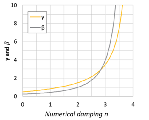
The numerical damping parameter n determines Newmark's integration parameters γ and β. The relationship between them is as follows:
Figure 9.5: Relationship between n, γ and β
| n | ρ∞ | β | γ |
| 0.0 | 1.00 | 0.25 | 0.50 |
| 0.5 | 0.75 | 0.33 | 0.64 |
| 1.0 | 0.50 | 0.44 | 0.83 |
| 1.5 | 0.25 | 0.64 | 1.10 |
| 2.0 | 0.00 | 1.00 | 1.50 |
| 2.5 | -0.25 | 1.78 | 2.17 |
| 3.0 | -0.50 | 4.00 | 3.50 |
| 3.5 | -0.75 | 16.00 | 7.50 |
Numerical damping is a property of the implicit time integration method, and this is an essential technique used in computational simulations of mechanical systems that exhibit discontinuities or chaotic behavior. It is implemented in numerical integrators to stabilize solutions and ensure convergence without sacrificing much accuracy. The method is particularly useful in systems where the eigenvalues are negative or excessively large, which are typically beyond the engineers' interest.
The primary purpose of numerical damping is to provide numerical stability. Numerical damping works by modifying the integration process to filter out responses that are outside the engineers' interest, effectively ignoring significant oscillations or discontinuities that could destabilize the computation. Especially, there are some characteristics of numerical damping.
Suppress High Frequency Noise: High-frequency components are more susceptible to numerical errors and can lead to instability in the solution. Numerical damping helps in smoothing out these components, thereby enhancing the overall stability of the integration scheme.
Preserves Low-Frequency Responses: These responses are crucial for accurate results in most engineering applications and need to be resolved with minimal alteration.
Maintain Stability with Large Time Steps: By damping out the higher frequencies, the integrator allows for larger time steps without sacrificing stability. This is especially useful for simulations where computational efficiency is important for long analysis end times and engineers are not concerned with high frequency responses.
Preventing Unphysical Oscillations: In dynamic simulations, especially those involving complex contact or boundary conditions, unphysical oscillations can occur. Numerical damping helps in mitigating these oscillations, ensuring the physical fidelity of the simulation.
Effects of Integration Step Size and Numerical Damping
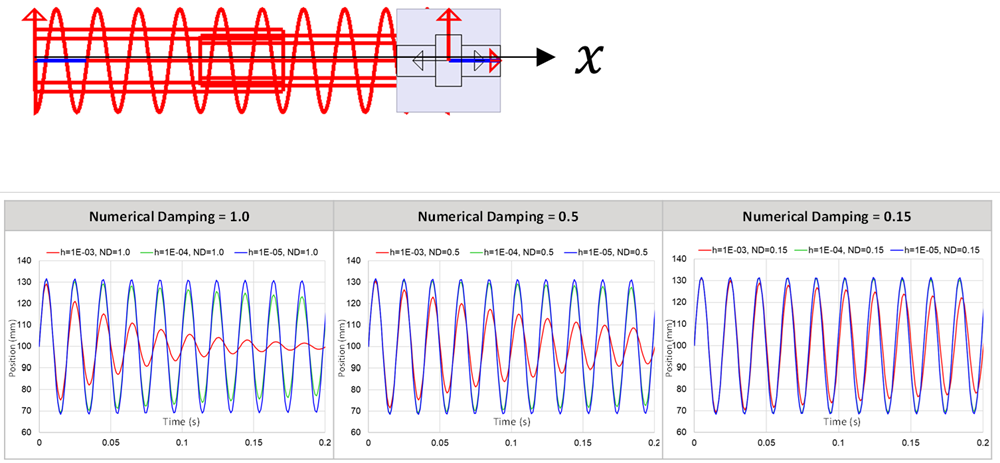
Numerical damping is influenced by the integration step size and numerical damping parameter n. As the step size decreases, and as the numerical damping parameter n is reduced, the effect of numerical damping lessens, which can enhance the accuracy of the simulation by reducing artificial energy dissipation that is not inherent to the physical system being modeled. If the numerical damping parameter n is set to 0, it results in minimal damping. Conversely, as the step size increases and the numerical damping parameter n increases, the numerical damping effect increases, thereby enhancing numerical stability. The default value of n is typically set to 1, which generally provides a balance between numerical stability and accuracy for standard problems.
In scenarios where comparisons with analytical solutions are desired, or in cases where the damping effects are crucial to the dynamics of the system, such as in studies of resonance phenomena or critical speeds in rotating machinery, it is advisable to set n to a lower value and reduce the maximum step size. This approach helps to maintain the physical fidelity of the simulation by minimizing numerical artifacts. Consequently, it is of paramount importance to set the correct numerical damping parameters and select an appropriate step size in order to guarantee that the simulation remains stable without any loss of accuracy.
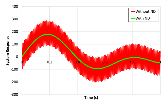
To illustrate, the figure below shows the effect of step size and numerical damping when a simple system consisting of a single body and spring (no physical damping) is simulated using Ansys Motion. With the default numerical damping parameter, the system's response shows minimal oscillation decay when using an extremely small step size (for example, 1E-5s). As the step size increases, the damping effect becomes more pronounced, leading to a greater reduction in oscillation amplitude. For a given numerical damping parameter, the damping ratio is proportional to the integration step size divided by the period of the system response. If the step size is reduced to 1/10 for a single period, the damping ratio also decreases to 1/10. As the numerical damping decreases, the effects of numerical damping become less pronounced, even with a large step size.
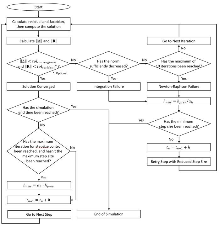
Motion employs the Newton-Raphson (NR) method to solve the nonlinear equations that represent the dynamics of a system accurately. The Motion solver dynamically adjusts the time steps based on the convergence or failure of the NR iterations, optimizing the analysis process for efficiency and accuracy.
The Motion Solver utilizes two primary convergence conditions: Displacement convergence and Residual convergence. Depending on the analysis settings, the solver may require both conditions to be satisfied to consider the iterations converged, or it may accept convergence when only the Displacement Convergence condition is met.
During NR iterations, the solver monitors the change in unknown variables, such as the position of a body. This condition is termed as Displacement Convergence. The criteria for assessing Displacement Convergence are the delta norm and the error tolerance for NR convergence:
- Delta Norm
Represents the norm of the generalized coordinate increments during NR iterations, indicating the magnitude of displacement changes. A higher delta norm suggests insufficient convergence of the unknown variables, which could signal issues in modeling or the need for smaller time steps.
- Error Tolerance for NR Convergence
If the delta norm is less than the error tolerance, set by default to 0.001, the solver deems the displacement to have sufficiently converged. Failure to reduce below this threshold may result in the solver reducing the step size to improve accuracy.
Residuals in the solver context refer to the unbalanced forces or moments that the solver attempts to minimize. If the Error tolerance factor for NR residual option is enabled in the analysis settings, the solver checks if the residual norm is sufficiently small to declare solution convergence. This condition is termed Residual Convergence.
- Residual Norm
Like the delta norm, this is the norm of the residuals during the iterations, which should decrease as the solver approaches a solution. A high residual norm indicates that the forces or moments have not sufficiently converged. If the residual norm does not decrease sufficiently during the NR iteration process, the solver may conclude that the NR has failed and can reduce the step size.
- Error tolerance for NR residual
A residual norm below this value indicates convergence. This value is calculated as:

(9–25)
where:
tolconvergence = Error tolerance for NR convergence Factorresidual = Error tolerance factor for NR residual. This value is defined in the analysis settings. tolresidual = Error tolerance for NR residual αresidual = An internal scaling factor, preset to 0.01
When using the residual norm as a convergence criterion, it is particularly useful for achieving higher accuracy in simulations of models with high stiffness or large force changes relative to small positional changes. Reducing the error tolerance factor for the NR residual value tightens the convergence criteria, potentially yielding more accurate solutions. However, this may also increase computational effort.
If the solver frequently fails to meet the convergence criteria due to the residual, disabling Error tolerance factor for NR residual option in the analysis settings can relax the convergence checks and improve solver performance.
Note: The Motion solver may not adhere to the convergence criteria mentioned above in order to achieve a more accurate solution or for the efficiency of the analysis process.
The criteria for determining that the solver has failed NR iteration are as follows:
- Integration Failure (IFAIL)
During the analysis, if the norm values do not decrease sufficiently, the solver can determine it as a convergence failure. This failure results in an increase in the IFAIL count.
- Newton-Raphson Failure (NFAIL)
If convergence criteria are not met after a maximum of 10 iterations, the solver is deemed to have failed, increasing the NRFAIL count.
If either IFAIL or NFAIL occurs, and the residual convergence condition remains unsatisfied, a Residual Failure (RFAIL) count is incremented. The counts for IFAIL, NFAIL, and RFAIL are output to the msg file.
Adaptive time stepping is a strategy that dynamically adjusts the time step size during a simulation based on the success or failure of NR iterations. The solver starts with the initial step size defined in the analysis settings and dynamically adjusts the step size during the analysis based on the success or failure of the NR iterations.
Reducing Time Step Size
When the solver in Motion fails to converge, it attempts to increase the likelihood of successful convergence in subsequent iterations by reducing the time step size. The new time step size for further attempts is calculated as follows:
 | (9–26) |
where:
| hnew = new step size |
| αh = step size factor, defined in the analysis settings |
| hprev = previous step size |
If the step size reaches the minimum step size (default: 1.0E-8 s), the
analysis will stop with an error stating, Minimum step size is
reached.
Increasing Time Step Size
If NR iterations converge easily, indicating less complex dynamics, the time step size can be increased without compromising accuracy to speed up the simulation process. If the NR iteration is successful for a number of consecutive iterations greater than the value set for Maximum iteration for stepsize control in the analysis settings, the solver may increase the time step. However, the solver will monitor delta and residual norm values to avoid increases that are likely to lead to NR failure. The increment will not be increased beyond the maximum increment. When conditions are met to increase the step size, it is adjusted as follows:
 | (9–27) |
The Include Static Analysis option is designed to perform a static analysis prior to the dynamic analysis, allowing the dynamic analysis to start from a static equilibrium position. For example, if it's desired to start the analysis from a static equilibrium position and consider initial deflection caused by self-weight or initial applied load conditions, this option can be used. For more information, see the Static Analysis.
The Include Eigenvalue Analysis option allows you to perform system eigenvalue analysis during dynamic analysis. When eigenvalue analysis is performed, the positions of bodies and nodes, as well as the stiffness of elements and springs, reflect the current state during dynamic analysis. Therefore, it can be effectively used to analyze how the mode shapes of a mechanical system change during operation.
Eigenvalue analysis is performed once at the beginning of the dynamic analysis when this option is enabled. If the number of eigenvalue analysis steps is greater than one, the analysis is performed at specified intervals throughout the simulation. The eigenvalue analysis interval, referred to as the eigenvalue analysis time step, is calculated using the formula:
 | (9–28) |
where:
| hi.eig = include eigenvalue analysis time step |
| Ni.eig = include eigenvalue analysis step (user defined) |
| Tend = simulation end time |
If include eigenvalue analysis option is activated so body eigenvalue analysis results are included in the dynamic analysis results, mode contribution analysis can be performed based on this. See Mode Contribution Analysis for more details.
The stabilization time option is utilized to expedite the assembly body's attainment of its initial state, specifically its static equilibrium position, within a designated timeframe. When enabled in the analysis settings, this option introduces artificial damping into the body's dynamics and stabilizes the acceleration arbitrarily, thereby facilitating rapid solution convergence towards the static equilibrium position. It is critical to understand that analyzing results during and immediately following the stabilization time is not advisable. Actual analysis scenarios that are necessary for driving the mechanical system, such as input motions, should commence only after the stabilization time. For example, in applications like a chained system where the goal is to determine the initial position of a chain influenced by its weight, this option can significantly reduce chain oscillations and swiftly achieve static equilibrium.
Eigenvalue analysis, also referred to as modal analysis, is a fundamental technique for the diagnostic and preventive analysis of vibrational issues in mechanical systems. It is employed to calculate the eigenvalues and eigenvectors, or the frequency response, of a system, enabling engineers to identify natural frequencies and corresponding mode shapes (eigenvectors). This identification is essential for detecting and avoiding resonance conditions that could lead to system failure. The insights gained from modal analysis are instrumental in designing more robust systems and enhancing the performance and durability of existing structures by allowing for the strategic modification of system parameters to achieve desired dynamic behaviors. Eigenvalue analysis therefore ensures the reliability and safety of various engineering applications, from optimizing vehicle suspension systems to designing earthquake-resistant buildings.
Note: Eigenvalue analysis might be computationally intensive, especially when the system includes nodal flexible bodies or nodal EasyFlex bodies, potentially leading to memory shortage errors. To mitigate such issues, transitioning the body to a modal flexible body representation could enable successful analysis completion by reducing memory demands.
This type of analysis is used to determine natural frequencies and mode shapes. In this process, the system's stiffness and mass properties are linearized and assumed to be constant throughout the analysis, even in the presence of nonlinear elements such as contacts and forces. Eigenvalue analysis can be conducted independently, utilizing stiffness properties based on the system's initial conditions, or during a dynamic analysis, where it reflects the stiffness properties at the specific instance of the analysis. Also, no damping effects are assumed in the eigenvalue analysis. The equation of motion for an undamped system is:
 | (9–29) |
where:
| M = mass matrix of the system |
| K = stiffness matrix of the system |
For a linear system, free vibrations will be harmonic of the form:
 | (9–30) |
where:
| Ψi = eigenvector representing the mode shape of the i-th natural frequency |
| ωi = i-th natural frequency (radians per unit time) |
| t = time |
Therefore, Equation 9–29 becomes:
 | (9–31) |
where:
| λi = ith eigenvalue |
The relationship between natural frequency and eigenvalue is:
 | (9–32) |
Equation 9–31 is satisfied if either Ψi=0 or if the determinant of (-λiM+K) is zero. The first option is the trivial one and, therefore, is not of interest. Thus, the second one gives the governing equations of the eigenvalue analysis:
Eigenvalue problem:
 | (9–33) |
Mass normalization:
 | (9–34) |
Stiffness normalization:
 | (9–35) |
The natural frequencies expressed in Hertz is:
 | (9–36) |
where:
| fi = ith natural frequency (cycles per unit time) |
This is an eigenvalue problem that can be solved for up to n values of λ and n eigenvectors Ψi which satisfying Equation 9–31, where n is the desired number of modes to extract. To solve for the eigenvalues λ and corresponding eigenvectors Ψi, the Arnoldi iteration is used, which is particularly effective for large, sparse, or structured matrices. This method is a generalization of the Lanczos method, designed to handle non-symmetric matrices, and it simplifies the extraction of the most significant modes from complex systems. This method allows the efficient extraction of a few significant modes (eigenvalues and eigenvectors) from large systems. This approach is particularly useful when only the most significant eigenvalues and eigenvectors are needed, rather than the full set.
Body Eigenvalue Analysis is used to calculate the eigenvalues and eigenvectors of a body. It is applicable to both nodal FE bodies and rigid bodies, with rigid bodies being treated as nodal EasyFlex bodies. An important output of this analysis is the generation of modal data in the form of a DFMF file. This can be used to convert an FE or EasyFlex body to a modal body type that uses modal synthesis. The governing equation is the same as for eigenvalue analysis in Equation 9–33 to Equation 9–35.
Body eigenvalue analysis supports two types of mode analysis, and .
- Normal Mode
The analysis calculates the body's eigenvalues under free-free boundary conditions. This mode is pivotal for determining the natural frequencies and mode shapes of a structure, devoid of external constraints. It primarily explores the inherent vibratory characteristics of the system, which is critical for predicting dynamic behaviors and enhancing structural designs by identifying potential resonances.
- With Static Correction Mode
, also known as , refines the eigenvalue calculation by incorporating static deformations. These deformations are induced by imposing unit displacements at specific nodal coordinates, which are defined by Rigid Body Elements (RBEs). Also known as the (CMS) method, this mode integrates the static responses due to specified displacements, therefore offering a more nuanced depiction of local deformations triggered by applied forces. This detailed representation helps in accurately assessing both the dynamic and static characteristics of the structure, making it exceptionally useful for analyzing structural responses where local flexibility and load paths play a crucial role in influencing the overall dynamic behavior.
System Eigenvalue Analysis is employed to evaluate the eigenvalues and eigenvectors not of individual bodies but of the entire system. Unlike body eigenvalue analysis, which focuses on single bodies or isolated components, system eigenvalue analysis assesses how interconnected components within the system influence its overall dynamic behavior. Through the analysis of derived vibration modes and natural frequencies, the interaction between different parts is elucidated. These interactions can significantly impact the system's performance and stability. In scenarios where parts are in contact, it is assumed that the contact point and the patch are connected by contact stiffness. The governing equation is the same as for eigenvalue analysis in Equation 9–33 to Equation 9–35.
Thermal analysis can be used to calculate the temperature, thermal strain, and stress of a body under heat conduction and convection. Nodal FE and nodal EasyFlex bodies are available in this analysis.
The governing equations for the steady state thermal analysis can be represented by the following equation.
 | (9–37) |
In general, the thermal conductivity matrix can be calculated as:
 | (9–38) |
The nodal thermal strain is:
 | (9–39) |
where:
| t = nodal temperature vector |
| tref = reference temperature |
| Δt = changes of nodal temperature vector in the NR iteration |
| K = thermal conductivity matrix of the bodies |
| Q = nodal heat flow vector such as heat flow input, convection, internal heat generation |
| B = partial derivatives of the shape function |
| k = conductivity matrix |
| εth = nodal thermal strain |
| α = thermal strain |
In transient thermal analysis, the heat capacity effect is required in the steady-state thermal analysis. The governing equations for the transient thermal analysis can be represented by the following equations.
(9–40) |
(9–41) |
The heat capacity matrix C can be calculated as:
(9–42) |
where:
| C = heat capacity matrix |
| α = coefficients of the integrator |
| ρ = density |
| c = specific heat |
| N = shape function |